spiketools
Utilities for converting, analyzing, and transforming spike trains.
The package uses one canonical spike-train representation throughout:
spiketimes.shape == (2, n_spikes)
spiketimes[0] contains spike times in milliseconds.
spiketimes[1] contains integer trial or unit indices.
The representation is intentionally simple so it can bridge different simulation backends, as long as the source data already represents spike events rather than persistent activity states:
- NEST events:
np.vstack([events["times"], events["senders"] - sender_offset]) - Binned spike-count matrices:
binary_to_spiketimes(spike_count_matrix, time_axis_ms) - BinaryNetwork diff logs in this repository:
BinaryNetwork.extract_spike_events_from_diff_logs(...) - Trial-wise Python lists:
spiketimes_to_list(spiketimes)
Empty trials are preserved with placeholder columns [nan, trial_id]. This
allows downstream trial-wise statistics to keep the original population size
even when some trials or neurons do not spike.
Persistent binary network states are a different datatype. A state matrix keeps
neurons at 1 until they switch off again, whereas spiketimes encodes only
event onsets. Converting state matrices to spike trains therefore requires an
explicit onset extraction step and is not what binary_to_spiketimes(...)
does.
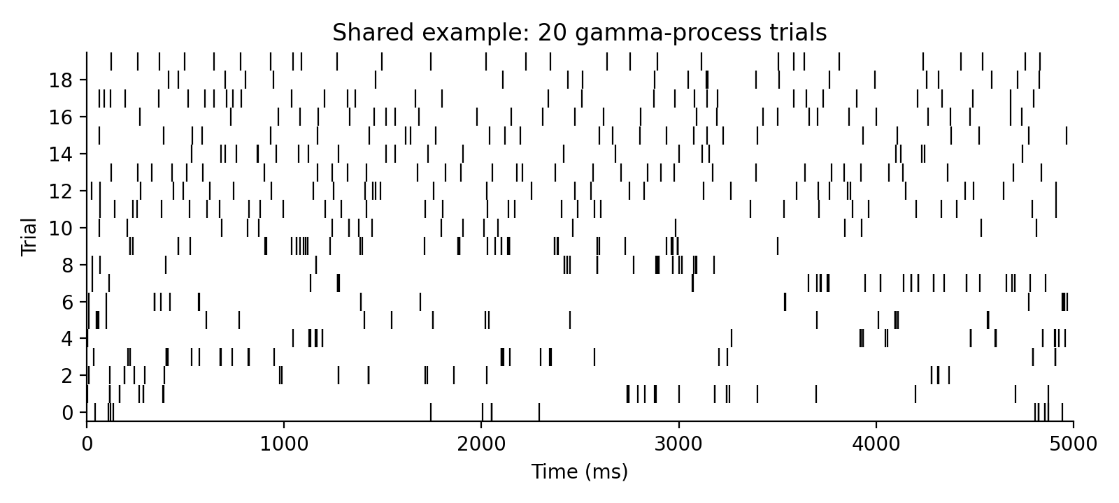
Shared Example Dataset
The examples below reuse one synthetic spike-train dataset: 20 trials, each
5 seconds long. Trials 0-9 share the same rate and a bursty gamma order
0.2 for controlled Fano-factor examples, while trials 10-19 use rates near
6 spikes/s and more regular orders for the interval-variability examples.
import numpy as np

from spiketools import gamma_spikes

np.random.seed(0)
rates = np.array([6.0] * 10 + [5.6, 6.3, 5.9, 6.5, 5.8, 6.1, 5.7, 6.4, 6.0, 5.5], dtype=float)
orders = np.array([0.2] * 10 + [1.0, 2.0, 2.0, 3.0, 1.0, 2.0, 3.0, 2.0, 1.0, 3.0], dtype=float)
spiketimes = gamma_spikes(rates=rates, order=orders, tlim=[0.0, 5000.0], dt=1.0)
Cookbook
Convert the shared example to a binned raster and a per-trial list:
import numpy as np

from spiketools import spiketimes_to_binary, spiketimes_to_list

binary, time = spiketimes_to_binary(spiketimes, tlim=[0.0, 5000.0], dt=50.0)
trials = spiketimes_to_list(spiketimes)
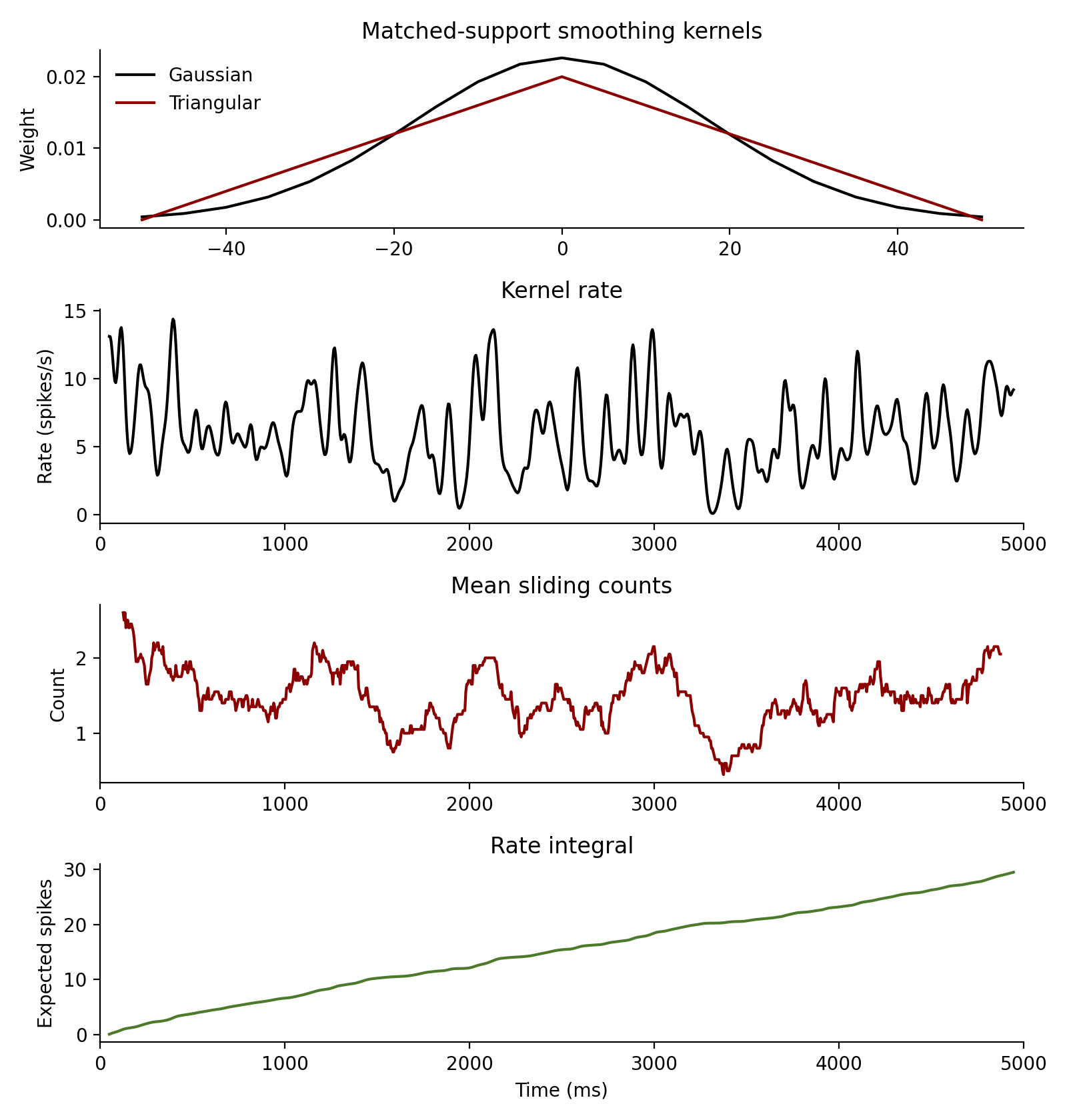
Estimate smoothed rates from the same spike trains:
from spiketools import gaussian_kernel, kernel_rate, rate_integral, sliding_counts, triangular_kernel

gauss = gaussian_kernel(25.0, dt=5.0, nstd=2.0)
# Match the Gaussian cutoff at +/- 50 ms on the dt = 5 ms grid.
tri = triangular_kernel((25.0 * 2.0) / (np.sqrt(6.0) * 5.0), dt=5.0)
rates, rate_time = kernel_rate(
    spiketimes,
    gauss,
    tlim=[0.0, 5000.0],
    dt=5.0,
    pool=True,
)
counts, count_time = sliding_counts(spiketimes, window=250.0, dt=5.0, tlim=[0.0, 5000.0])
integrated = rate_integral(rates[0], dt=5.0)
Compute trial-wise variability metrics:
from spiketools.variability import cv2, cv_two, ff

trial_id = 13
trial = spiketimes[:, spiketimes[1] == trial_id].copy()
trial[1] = 0
ff_trials = spiketimes[:, spiketimes[1] < 10].copy()

print(f"Trial {trial_id} uses gamma order {orders[trial_id]}; expect cv2 < 1.")
print(round(float(cv2(trial)), 3))
print(round(float(cv_two(trial, min_vals=2)), 3))
print("Trials 0-9 use rate 6 spikes/s and gamma order 0.2; expect ff > 1.")
print(round(float(ff(ff_trials, tlim=[0.0, 5000.0])), 3))
Example output:
Trial 13 uses gamma order 3.0; expect cv2 < 1.
0.292
0.536
Trials 0-9 use rate 6 spikes/s and gamma order 0.2; expect ff > 1.
2.891
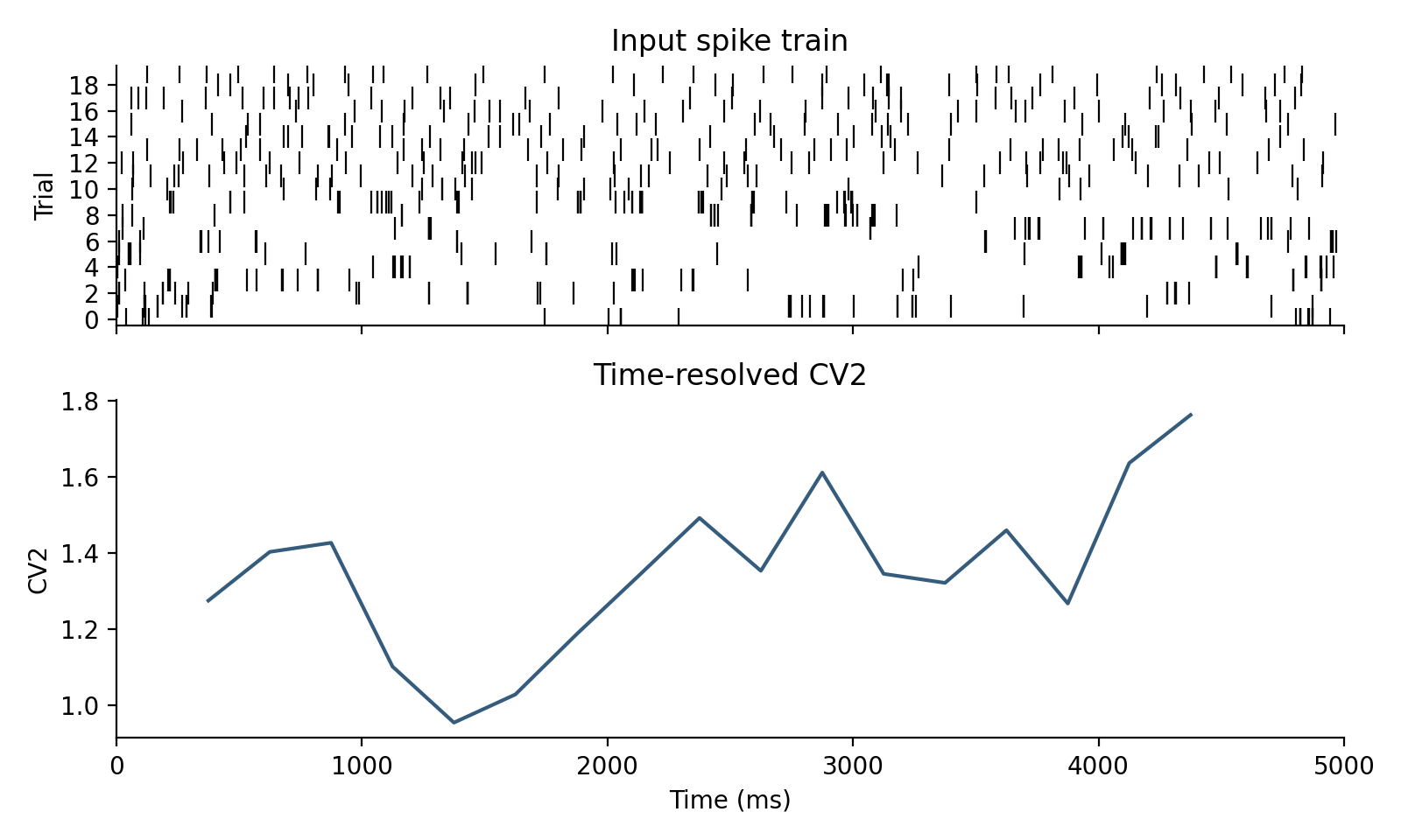
Run a sliding-window analysis on the same dataset:
from spiketools import time_resolved
from spiketools.variability import cv2

values, window_time = time_resolved(
    spiketimes,
    window=1000.0,
    func=cv2,
    kwargs={"pool": True},
    tlim=[0.0, 5000.0],
    tstep=250.0,
)

print(np.round(values[:5], 3))
print(np.round(window_time[:5], 1))
Example output:
[1.276 1.404 1.427 1.102 0.955]
[ 375.  625.  875. 1125. 1375.]
Regenerating docs:
python scripts/generate_api_docs.py
1"""Utilities for converting, analyzing, and transforming spike trains. 2 3The package uses one canonical spike-train representation throughout: 4 5`spiketimes.shape == (2, n_spikes)` 6 `spiketimes[0]` contains spike times in milliseconds. 7 `spiketimes[1]` contains integer trial or unit indices. 8 9The representation is intentionally simple so it can bridge different 10simulation backends, as long as the source data already represents spike 11events rather than persistent activity states: 12 13- NEST events: 14 `np.vstack([events["times"], events["senders"] - sender_offset])` 15- Binned spike-count matrices: 16 `binary_to_spiketimes(spike_count_matrix, time_axis_ms)` 17- BinaryNetwork diff logs in this repository: 18 `BinaryNetwork.extract_spike_events_from_diff_logs(...)` 19- Trial-wise Python lists: 20 `spiketimes_to_list(spiketimes)` 21 22Empty trials are preserved with placeholder columns `[nan, trial_id]`. This 23allows downstream trial-wise statistics to keep the original population size 24even when some trials or neurons do not spike. 25 26Persistent binary network states are a different datatype. A state matrix keeps 27neurons at `1` until they switch off again, whereas `spiketimes` encodes only 28event onsets. Converting state matrices to spike trains therefore requires an 29explicit onset extraction step and is not what `binary_to_spiketimes(...)` 30does. 31 32Shared Example Dataset 33---------------------- 34 35The examples below reuse one synthetic spike-train dataset: `20` trials, each 36`5` seconds long. Trials `0-9` share the same rate and a bursty gamma order 37`0.2` for controlled Fano-factor examples, while trials `10-19` use rates near 38`6 spikes/s` and more regular orders for the interval-variability examples. 39 40```python 41import numpy as np 42 43from spiketools import gamma_spikes 44 45np.random.seed(0) 46rates = np.array([6.0] * 10 + [5.6, 6.3, 5.9, 6.5, 5.8, 6.1, 5.7, 6.4, 6.0, 5.5], dtype=float) 47orders = np.array([0.2] * 10 + [1.0, 2.0, 2.0, 3.0, 1.0, 2.0, 3.0, 2.0, 1.0, 3.0], dtype=float) 48spiketimes = gamma_spikes(rates=rates, order=orders, tlim=[0.0, 5000.0], dt=1.0) 49``` 50 51 52 53Cookbook 54-------- 55 56Convert the shared example to a binned raster and a per-trial list: 57 58```python 59import numpy as np 60 61from spiketools import spiketimes_to_binary, spiketimes_to_list 62 63binary, time = spiketimes_to_binary(spiketimes, tlim=[0.0, 5000.0], dt=50.0) 64trials = spiketimes_to_list(spiketimes) 65``` 66 67Estimate smoothed rates from the same spike trains: 68 69```python 70from spiketools import gaussian_kernel, kernel_rate, rate_integral, sliding_counts, triangular_kernel 71 72gauss = gaussian_kernel(25.0, dt=5.0, nstd=2.0) 73# Match the Gaussian cutoff at +/- 50 ms on the dt = 5 ms grid. 74tri = triangular_kernel((25.0 * 2.0) / (np.sqrt(6.0) * 5.0), dt=5.0) 75rates, rate_time = kernel_rate( 76 spiketimes, 77 gauss, 78 tlim=[0.0, 5000.0], 79 dt=5.0, 80 pool=True, 81) 82counts, count_time = sliding_counts(spiketimes, window=250.0, dt=5.0, tlim=[0.0, 5000.0]) 83integrated = rate_integral(rates[0], dt=5.0) 84``` 85 86 87 88Compute trial-wise variability metrics: 89 90```python 91from spiketools.variability import cv2, cv_two, ff 92 93trial_id = 13 94trial = spiketimes[:, spiketimes[1] == trial_id].copy() 95trial[1] = 0 96ff_trials = spiketimes[:, spiketimes[1] < 10].copy() 97 98print(f"Trial {trial_id} uses gamma order {orders[trial_id]}; expect cv2 < 1.") 99print(round(float(cv2(trial)), 3)) 100print(round(float(cv_two(trial, min_vals=2)), 3)) 101print("Trials 0-9 use rate 6 spikes/s and gamma order 0.2; expect ff > 1.") 102print(round(float(ff(ff_trials, tlim=[0.0, 5000.0])), 3)) 103``` 104 105Example output: 106 107```text 108Trial 13 uses gamma order 3.0; expect cv2 < 1. 1090.292 1100.536 111Trials 0-9 use rate 6 spikes/s and gamma order 0.2; expect ff > 1. 1122.891 113``` 114 115Run a sliding-window analysis on the same dataset: 116 117```python 118from spiketools import time_resolved 119from spiketools.variability import cv2 120 121values, window_time = time_resolved( 122 spiketimes, 123 window=1000.0, 124 func=cv2, 125 kwargs={"pool": True}, 126 tlim=[0.0, 5000.0], 127 tstep=250.0, 128) 129 130print(np.round(values[:5], 3)) 131print(np.round(window_time[:5], 1)) 132``` 133 134Example output: 135 136```text 137[1.276 1.404 1.427 1.102 0.955] 138[ 375. 625. 875. 1125. 1375.] 139``` 140 141 142 143Regenerating docs: 144 145```bash 146python scripts/generate_api_docs.py 147``` 148""" 149 150from __future__ import annotations 151 152from . import conversion, population, rate, surrogates, transforms, variability, windowing 153from .conversion import ( 154 binary_to_spiketimes, 155 cut_spiketimes, 156 get_time_limits, 157 spiketimes_to_binary, 158 spiketimes_to_list, 159) 160from .population import synchrony 161from .rate import ( 162 gaussian_kernel, 163 kernel_rate, 164 rate_integral, 165 sliding_counts, 166 triangular_kernel, 167) 168from .surrogates import gamma_spikes 169from .transforms import resample, time_stretch, time_warp 170from .variability import ( 171 cv2, 172 cv_two, 173 ff, 174 lv, 175 kernel_fano, 176 time_resolved_cv2, 177 time_resolved_cv_two, 178 time_warped_cv2, 179) 180from .windowing import rate_warped_analysis, time_resolved, time_resolved_new 181 182__all__ = [ 183 # Submodules 184 "conversion", 185 "population", 186 "rate", 187 "surrogates", 188 "transforms", 189 "variability", 190 "windowing", 191 # Conversion utilities 192 "binary_to_spiketimes", 193 "cut_spiketimes", 194 "get_time_limits", 195 "spiketimes_to_binary", 196 "spiketimes_to_list", 197 # Rate analysis 198 "gaussian_kernel", 199 "kernel_rate", 200 "rate_integral", 201 "sliding_counts", 202 "triangular_kernel", 203 # Windowed analyses 204 "rate_warped_analysis", 205 "time_resolved", 206 "time_resolved_new", 207 # Variability analysis 208 "cv2", 209 "cv_two", 210 "ff", 211 "kernel_fano", 212 "lv", 213 "time_resolved_cv2", 214 "time_resolved_cv_two", 215 "time_warped_cv2", 216 # Transforms and helpers 217 "resample", 218 "time_stretch", 219 "time_warp", 220 # Population-level metrics 221 "synchrony", 222 # Surrogate generation 223 "gamma_spikes", 224]
137def binary_to_spiketimes(binary: np.ndarray, time: Iterable[float]) -> np.ndarray:
138    """
139    Convert a binned spike matrix into canonical `spiketimes`.
140
141    Parameters
142    ----------
143    binary:
144        Array with shape `(n_trials, n_bins)`. Values larger than `1` are
145        interpreted as multiple spikes in the same bin.
146    time:
147        One time value per bin, typically the left bin edges in ms.
148
149    Returns
150    -------
151    np.ndarray
152        `float` array with shape `(2, n_spikes_or_markers)`.
153
154    Notes
155    -----
156    Trials with no spikes are retained via placeholder columns
157    `[nan, trial_id]`.
158
159    This function assumes that each non-zero entry denotes one or more spike
160    events in that time bin. It is not intended for persistent state matrices
161    where a neuron stays at `1` across consecutive bins until the next update.
162
163    Examples
164    --------
165    Convert a spike-count raster on a regular grid:
166
167    >>> binary_to_spiketimes(
168    ...     np.array([[1, 0, 2], [0, 0, 0]]),
169    ...     [0.0, 1.0, 2.0],
170    ... ).tolist()
171    [[0.0, 2.0, 2.0, nan], [0.0, 0.0, 0.0, 1.0]]
172    """
173    time = pylab.array(time)
174    spiketimes: list[list[float]] = [[], []]
175    max_count = binary.max()
176    spikes = binary.copy()
177    while max_count > 0:
178        if max_count == 1:
179            trial, t_index = spikes.nonzero()
180        else:
181            trial, t_index = pylab.where(spikes == max_count)
182        spiketimes[0] += time[t_index].tolist()
183        spiketimes[1] += trial.tolist()
184        spikes[spikes == max_count] -= 1
185        max_count -= 1
186    spiketimes_array = pylab.array(spiketimes)
187
188    all_trials = set(range(binary.shape[0]))
189    found_trials = set(spiketimes_array[1, :])
190    missing_trials = list(all_trials.difference(found_trials))
191    for mt in missing_trials:
192        spiketimes_array = pylab.append(
193            spiketimes_array, pylab.array([[pylab.nan], [mt]]), axis=1
194        )
195    return spiketimes_array.astype(float)
Convert a binned spike matrix into canonical spiketimes.
Parameters
- binary:: Array with shape
(n_trials, n_bins). Values larger than1are interpreted as multiple spikes in the same bin. - time:: One time value per bin, typically the left bin edges in ms.
Returns
- np.ndarray:
floatarray with shape(2, n_spikes_or_markers).
Notes
Trials with no spikes are retained via placeholder columns
[nan, trial_id].
This function assumes that each non-zero entry denotes one or more spike
events in that time bin. It is not intended for persistent state matrices
where a neuron stays at 1 across consecutive bins until the next update.
Examples
Convert a spike-count raster on a regular grid:
>>> binary_to_spiketimes(
...     np.array([[1, 0, 2], [0, 0, 0]]),
...     [0.0, 1.0, 2.0],
... ).tolist()
[[0.0, 2.0, 2.0, nan], [0.0, 0.0, 0.0, 1.0]]
239def cut_spiketimes(spiketimes: np.ndarray, tlim: Sequence[float]) -> np.ndarray:
240    """
241    Restrict `spiketimes` to a time interval.
242
243    Parameters
244    ----------
245    spiketimes:
246        Canonical spike representation.
247    tlim:
248        Two-element sequence `[tmin, tmax]` in ms. The interval is inclusive at
249        the start and exclusive at the end.
250
251    Returns
252    -------
253    np.ndarray
254        Cropped spike array. Empty trials are still represented by
255        `[nan, trial_id]` markers.
256
257    Examples
258    --------
259    >>> cut_spiketimes(
260    ...     np.array([[1.0, 3.0, 5.0], [0.0, 0.0, 1.0]]),
261    ...     [2.0, 5.0],
262    ... ).tolist()
263    [[3.0, nan], [0.0, 1.0]]
264    """
265    alltrials = list(set(spiketimes[1, :]))
266    cut_spikes = spiketimes[:, pylab.isfinite(spiketimes[0])]
267    cut_spikes = cut_spikes[:, cut_spikes[0, :] >= tlim[0]]
268
269    if cut_spikes.shape[1] > 0:
270        cut_spikes = cut_spikes[:, cut_spikes[0, :] < tlim[1]]
271    for trial in alltrials:
272        if trial not in cut_spikes[1, :]:
273            cut_spikes = pylab.append(
274                cut_spikes, pylab.array([[pylab.nan], [trial]]), axis=1
275            )
276    return cut_spikes
Restrict spiketimes to a time interval.
Parameters
- spiketimes:: Canonical spike representation.
- tlim:: Two-element sequence
[tmin, tmax]in ms. The interval is inclusive at the start and exclusive at the end.
Returns
- np.ndarray: Cropped spike array. Empty trials are still represented by
[nan, trial_id]markers.
Examples
>>> cut_spiketimes(
...     np.array([[1.0, 3.0, 5.0], [0.0, 0.0, 1.0]]),
...     [2.0, 5.0],
... ).tolist()
[[3.0, nan], [0.0, 1.0]]
45def get_time_limits(spiketimes: np.ndarray) -> list[float]:
46    """
47    Infer time limits from a `spiketimes` array.
48
49    Parameters
50    ----------
51    spiketimes:
52        Canonical spike representation with shape `(2, n_spikes)`.
53
54    Returns
55    -------
56    list[float]
57        `[tmin, tmax]` with inclusive start and exclusive end. If inference
58        fails, `[0.0, 1.0]` is returned as a safe fallback.
59
60    Examples
61    --------
62    >>> spikes = np.array([[5.0, 8.0], [0.0, 1.0]])
63    >>> get_time_limits(spikes)
64    [5.0, 9.0]
65    """
66    try:
67        tlim = [
68            float(pylab.nanmin(spiketimes[0, :])),
69            float(pylab.nanmax(spiketimes[0, :]) + 1),
70        ]
71    except Exception:
72        tlim = [0.0, 1.0]
73    if pylab.isnan(tlim).any():
74        tlim = [0.0, 1.0]
75    return tlim
Infer time limits from a spiketimes array.
Parameters
- spiketimes:: Canonical spike representation with shape
(2, n_spikes).
Returns
- list[float]:
[tmin, tmax]with inclusive start and exclusive end. If inference fails,[0.0, 1.0]is returned as a safe fallback.
Examples
>>> spikes = np.array([[5.0, 8.0], [0.0, 1.0]])
>>> get_time_limits(spikes)
[5.0, 9.0]
 78def spiketimes_to_binary(
 79    spiketimes: np.ndarray,
 80    tlim: Optional[Sequence[float]] = None,
 81    dt: float = 1.0,
 82) -> tuple[np.ndarray, np.ndarray]:
 83    """
 84    Convert `spiketimes` into a spike-count matrix on a regular time grid.
 85
 86    Parameters
 87    ----------
 88    spiketimes:
 89        Canonical spike representation. Row `0` stores times in ms, row `1`
 90        stores trial or unit indices.
 91    tlim:
 92        Two-element sequence defining [tmin, tmax] in ms. Defaults to inferred bounds.
 93    dt:
 94        Temporal resolution in ms.
 95
 96    Returns
 97    -------
 98    tuple[np.ndarray, np.ndarray]
 99        `(binary, time)` where `binary.shape == (n_trials, n_bins)` and
100        `time` contains the left bin edges in ms.
101
102    Notes
103    -----
104    The output is not strictly binary if multiple spikes land in the same bin.
105    In that case the matrix stores spike counts per bin.
106
107    Examples
108    --------
109    >>> spikes = np.array([[0.0, 1.0, 1.0], [0.0, 0.0, 1.0]])
110    >>> binary, time = spiketimes_to_binary(spikes, tlim=[0.0, 3.0], dt=1.0)
111    >>> binary.astype(int).tolist()
112    [[1, 1, 0], [0, 1, 0]]
113    >>> time.tolist()
114    [-0.5, 0.5, 1.5]
115    """
116    if tlim is None:
117        tlim = get_time_limits(spiketimes)
118
119    time = pylab.arange(tlim[0], tlim[1] + dt, dt).astype(float)
120    if dt <= 1:
121        time -= 0.5 * float(dt)
122
123    trials = pylab.array([-1] + list(range(int(spiketimes[1, :].max() + 1)))) + 0.5
124
125    tlim_spikes = cut_spiketimes(spiketimes, tlim)
126    tlim_spikes = tlim_spikes[:, pylab.isnan(tlim_spikes[0, :]) == False]
127
128    if tlim_spikes.shape[1] > 0:
129        binary = pylab.histogram2d(
130            tlim_spikes[0, :], tlim_spikes[1, :], [time, trials]
131        )[0].T
132    else:
133        binary = pylab.zeros((len(trials) - 1, len(time) - 1))
134    return binary, time[:-1]
Convert spiketimes into a spike-count matrix on a regular time grid.
Parameters
- spiketimes:: Canonical spike representation. Row
0stores times in ms, row1stores trial or unit indices. - tlim:: Two-element sequence defining [tmin, tmax] in ms. Defaults to inferred bounds.
- dt:: Temporal resolution in ms.
Returns
- tuple[np.ndarray, np.ndarray]:
(binary, time)wherebinary.shape == (n_trials, n_bins)andtimecontains the left bin edges in ms.
Notes
The output is not strictly binary if multiple spikes land in the same bin. In that case the matrix stores spike counts per bin.
Examples
>>> spikes = np.array([[0.0, 1.0, 1.0], [0.0, 0.0, 1.0]])
>>> binary, time = spiketimes_to_binary(spikes, tlim=[0.0, 3.0], dt=1.0)
>>> binary.astype(int).tolist()
[[1, 1, 0], [0, 1, 0]]
>>> time.tolist()
[-0.5, 0.5, 1.5]
198def spiketimes_to_list(spiketimes: np.ndarray) -> list[np.ndarray]:
199    """
200    Convert canonical `spiketimes` into one array per trial or unit.
201
202    Parameters
203    ----------
204    spiketimes:
205        Spike array with times in row `0` and indices in row `1`.
206
207    Returns
208    -------
209    list[np.ndarray]
210        `result[i]` contains the spike times of trial or unit `i`.
211
212    Examples
213    --------
214    >>> spiketimes_to_list(np.array([[1.0, 2.0, 4.0], [0.0, 1.0, 1.0]]))
215    [array([1.]), array([2., 4.])]
216    """
217    if spiketimes.shape[1] == 0:
218        return []
219    trials = range(int(spiketimes[1, :].max() + 1))
220    orderedspiketimes = spiketimes.copy()
221    orderedspiketimes = orderedspiketimes[
222        :, pylab.isnan(orderedspiketimes[0]) == False
223    ]
224    spike_order = pylab.argsort(orderedspiketimes[0], kind="mergesort")
225    orderedspiketimes = orderedspiketimes[:, spike_order]
226    trial_order = pylab.argsort(orderedspiketimes[1], kind="mergesort")
227    orderedspiketimes = orderedspiketimes[:, trial_order]
228
229    spikelist: list[Optional[np.ndarray]] = [None] * len(trials)
230    start = 0
231    for trial in trials:
232        end = bisect_right(orderedspiketimes[1], trial)
233        trialspikes = orderedspiketimes[0, start:end]
234        start = end
235        spikelist[trial] = trialspikes
236    return [spikes if spikes is not None else pylab.array([]) for spikes in spikelist]
Convert canonical spiketimes into one array per trial or unit.
Parameters
- spiketimes:: Spike array with times in row
0and indices in row1.
Returns
- list[np.ndarray]:
result[i]contains the spike times of trial or uniti.
Examples
>>> spiketimes_to_list(np.array([[1.0, 2.0, 4.0], [0.0, 1.0, 1.0]]))
[array([1.]), array([2., 4.])]
 88def gaussian_kernel(sigma, dt=1.0, nstd=3.0):
 89    r"""Return a normalized Gaussian kernel for rate smoothing.
 90
 91    Parameters
 92    ----------
 93    sigma:
 94        Kernel width in ms.
 95    dt:
 96        Temporal resolution of the target grid in ms.
 97    nstd:
 98        Half-width of the kernel in units of `sigma`.
 99
100    Definition
101    ----------
102    On a grid $t_k = k\,dt$ centered at zero, this function samples the
103    truncated Gaussian
104
105    $$
106    G_{\sigma, n_\mathrm{std}}(t) =
107    \begin{cases}
108    \frac{\exp\left(-(t / \sigma)^2\right)}
109    {\int_{-n_\mathrm{std}\sigma}^{n_\mathrm{std}\sigma} \exp\left(-(u / \sigma)^2\right)\,du}
110    & \text{for } |t| \le n_\mathrm{std}\,\sigma, \\
111    0 & \text{otherwise,}
112    \end{cases}
113    $$
114
115    and rescales the sampled support so that `kernel.sum() * dt = 1`.
116
117    <img src="spiketools_assets/gaussian_kernel_example.png"
118         alt="Gaussian kernel example"
119         onerror="this.onerror=null;this.src='../spiketools_assets/gaussian_kernel_example.png';" />
120
121    Examples
122    --------
123    >>> kernel = gaussian_kernel(2.0, dt=1.0, nstd=1.0)
124    >>> round(kernel.sum(), 3)
125    1.0
126    """
127    t = pylab.arange(-nstd * sigma, nstd * sigma + dt, dt)
128    gauss = pylab.exp(-t ** 2 / sigma ** 2)
129    gauss /= gauss.sum() * dt
130    return gauss
Return a normalized Gaussian kernel for rate smoothing.
Parameters
- sigma:: Kernel width in ms.
- dt:: Temporal resolution of the target grid in ms.
- nstd:: Half-width of the kernel in units of
sigma.
Definition
On a grid $t_k = k\,dt$ centered at zero, this function samples the truncated Gaussian
$$ G_{\sigma, n_\mathrm{std}}(t) = \begin{cases} \frac{\exp\left(-(t / \sigma)^2\right)} {\int_{-n_\mathrm{std}\sigma}^{n_\mathrm{std}\sigma} \exp\left(-(u / \sigma)^2\right)\,du} & \text{for } |t| \le n_\mathrm{std}\,\sigma, \ 0 & \text{otherwise,} \end{cases} $$
and rescales the sampled support so that kernel.sum() * dt = 1.
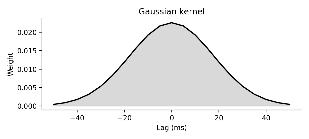
Examples
>>> kernel = gaussian_kernel(2.0, dt=1.0, nstd=1.0)
>>> round(kernel.sum(), 3)
1.0
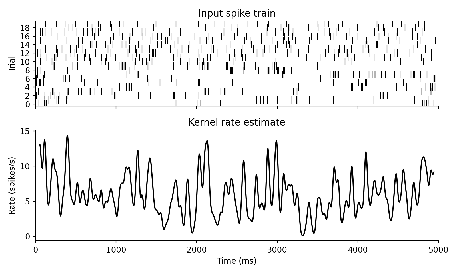
171def kernel_rate(spiketimes, kernel, tlim=None, dt=1.0, pool=True):
172    r"""Estimate smoothed firing rates from `spiketimes`.
173
174    Parameters
175    ----------
176    spiketimes:
177        Canonical spike representation with times in ms.
178    kernel:
179        One-dimensional kernel normalized to unit integral in seconds.
180    tlim:
181        Optional `[tmin, tmax]` interval in ms.
182    dt:
183        Bin width in ms used for discretization before convolution.
184    pool:
185        If `True`, average across trials or units before convolution and return
186        a single population rate trace. If `False`, return one trace per row.
187
188    Returns
189    -------
190    tuple[np.ndarray, np.ndarray]
191        `(rates, time)` where `rates` is in spikes/s.
192
193    Definition
194    ----------
195    If `b_i[k]` is the discretized spike train on row `i`, then the returned
196    estimate is the discrete kernel convolution
197
198    $$
199    r_i[n] = 1000 \sum_k b_i[k]\,K[n-k]
200    $$
201
202    where $K$ is normalized so that $\sum_k K[k]\,dt = 1$. If `pool=True`, the
203    mean spike train across rows is convolved before returning the result.
204
205    <img src="spiketools_assets/kernel_rate_example.png"
206         alt="Kernel rate example"
207         onerror="this.onerror=null;this.src='../spiketools_assets/kernel_rate_example.png';" />
208
209    Examples
210    --------
211    >>> spikes = np.array([[0.0, 2.0], [0.0, 0.0]])
212    >>> kernel = gaussian_kernel(1.0, dt=1.0, nstd=1.0)
213    >>> rates, time = kernel_rate(spikes, kernel, tlim=[0.0, 4.0], dt=1.0, pool=False)
214    >>> rates.shape, time.shape
215    ((1, 2), (2,))
216    """
217    if tlim is None:
218        tlim = get_time_limits(spiketimes)
219
220    binary, time = spiketimes_to_binary(spiketimes, tlim, dt)
221
222    if pool:
223        binary = binary.mean(axis=0)[pylab.newaxis, :]
224
225    rates = convolve2d(binary, kernel[pylab.newaxis, :], "same")
226    kwidth = len(kernel)
227    rates = rates[:, int(kwidth / 2) : -int(kwidth / 2)]
228    time = time[int(kwidth / 2) : -int(kwidth / 2)]
229    return rates * 1000.0, time
Estimate smoothed firing rates from spiketimes.
Parameters
- spiketimes:: Canonical spike representation with times in ms.
- kernel:: One-dimensional kernel normalized to unit integral in seconds.
- tlim:: Optional
[tmin, tmax]interval in ms. - dt:: Bin width in ms used for discretization before convolution.
- pool:: If
True, average across trials or units before convolution and return a single population rate trace. IfFalse, return one trace per row.
Returns
- tuple[np.ndarray, np.ndarray]:
(rates, time)whereratesis in spikes/s.
Definition
If b_i[k] is the discretized spike train on row i, then the returned
estimate is the discrete kernel convolution
$$ r_i[n] = 1000 \sum_k b_i[k]\,K[n-k] $$
where $K$ is normalized so that $\sum_k K[k]\,dt = 1$. If pool=True, the
mean spike train across rows is convolved before returning the result.
Examples
>>> spikes = np.array([[0.0, 2.0], [0.0, 0.0]])
>>> kernel = gaussian_kernel(1.0, dt=1.0, nstd=1.0)
>>> rates, time = kernel_rate(spikes, kernel, tlim=[0.0, 4.0], dt=1.0, pool=False)
>>> rates.shape, time.shape
((1, 2), (2,))
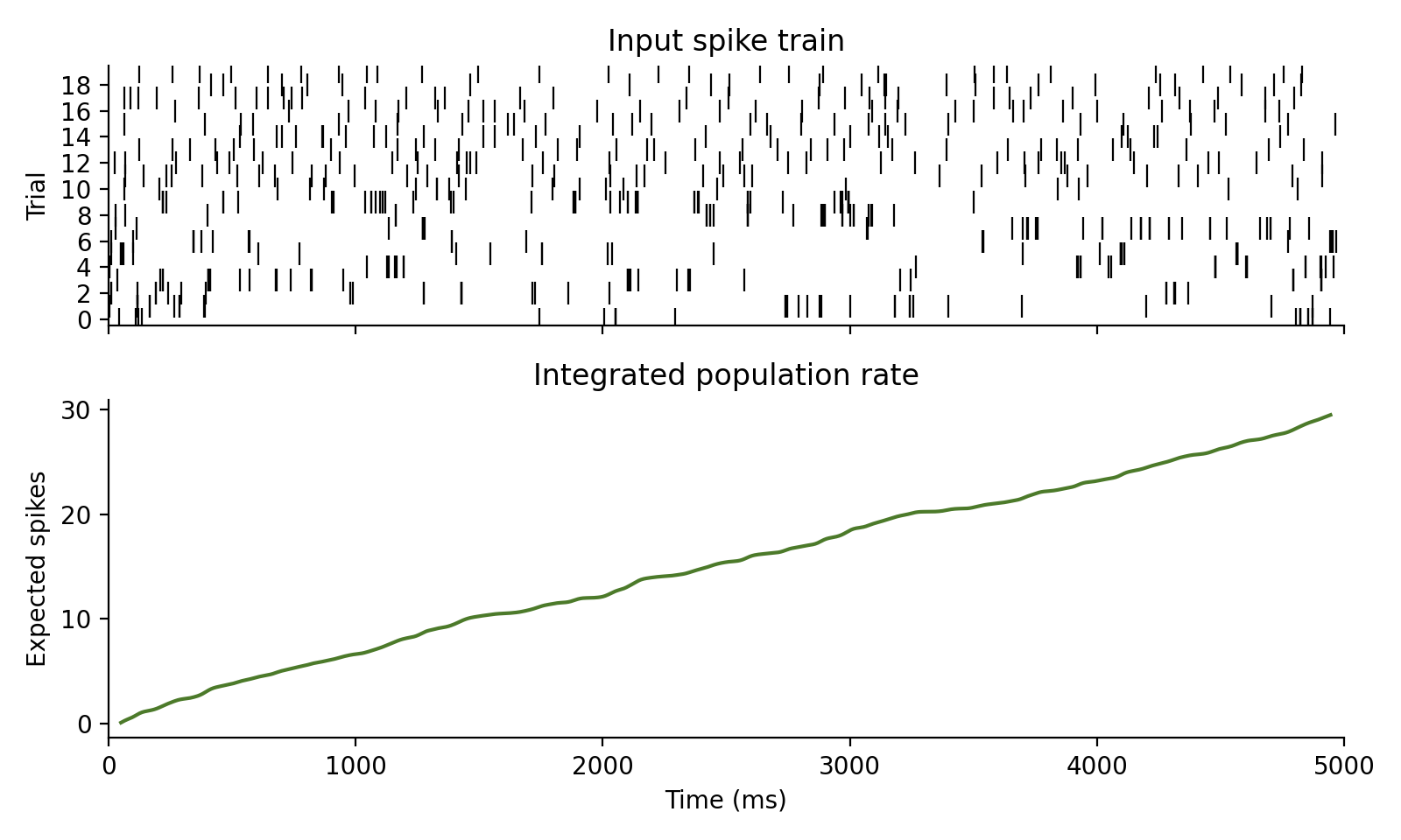
281def rate_integral(rate, dt):
282    r"""Integrate a rate trace in spikes/s to expected spike counts.
283
284    Parameters
285    ----------
286    rate:
287        One-dimensional rate trace in spikes/s.
288    dt:
289        Sampling interval in ms.
290
291    Definition
292    ----------
293    The cumulative expected spike count is
294
295    $$
296    I[n] = \sum_{k \le n} r[k]\,dt / 1000
297    $$
298
299    which is the discrete-time version of integrating the rate over time.
300
301    <img src="spiketools_assets/rate_integral_example.png"
302         alt="Rate integral example"
303         onerror="this.onerror=null;this.src='../spiketools_assets/rate_integral_example.png';" />
304
305    Examples
306    --------
307    >>> rate_integral(np.array([500.0, 500.0]), dt=1.0).tolist()
308    [0.5, 1.0]
309    """
310    return pylab.cumsum(rate / 1000.0) * dt
Integrate a rate trace in spikes/s to expected spike counts.
Parameters
- rate:: One-dimensional rate trace in spikes/s.
- dt:: Sampling interval in ms.
Definition
The cumulative expected spike count is
$$ I[n] = \sum_{k \le n} r[k]\,dt / 1000 $$
which is the discrete-time version of integrating the rate over time.
Examples
>>> rate_integral(np.array([500.0, 500.0]), dt=1.0).tolist()
[0.5, 1.0]
232def sliding_counts(spiketimes, window, dt=1.0, tlim=None):
233    r"""Count spikes inside a sliding window.
234
235    Parameters
236    ----------
237    spiketimes:
238        Canonical spike representation.
239    window:
240        Window width in ms.
241    dt:
242        Step size of the discretized binary representation in ms.
243    tlim:
244        Optional `[tmin, tmax]` interval in ms.
245
246    Definition
247    ----------
248    With $W = \text{window} / dt$ bins and binned spike train `b_i[k]`, this function
249    returns
250
251    $$
252    C_i[n] = \sum_{k = 0}^{W - 1} b_i[n + k]
253    $$
254
255    for each row `i`.
256
257    <img src="spiketools_assets/sliding_counts_example.png"
258         alt="Sliding counts example"
259         onerror="this.onerror=null;this.src='../spiketools_assets/sliding_counts_example.png';" />
260
261    Examples
262    --------
263    >>> spikes = np.array([[0.0, 2.0], [0.0, 0.0]])
264    >>> counts, time = sliding_counts(spikes, window=2.0, dt=1.0, tlim=[0.0, 4.0])
265    >>> counts.astype(int).tolist()
266    [[1, 1, 1]]
267    """
268    if tlim is None:
269        tlim = get_time_limits(spiketimes)
270    binary, time = spiketimes_to_binary(spiketimes, dt=dt, tlim=tlim)
271
272    kernel = pylab.ones((1, int(window // dt)))
273    counts = convolve2d(binary, kernel, "valid")
274
275    dif = time.shape[0] - counts.shape[1]
276    time = time[int(np.ceil(dif / 2)) : int(-dif / 2)]
277
278    return counts, time
Count spikes inside a sliding window.
Parameters
- spiketimes:: Canonical spike representation.
- window:: Window width in ms.
- dt:: Step size of the discretized binary representation in ms.
- tlim:: Optional
[tmin, tmax]interval in ms.
Definition
With $W = \text{window} / dt$ bins and binned spike train b_i[k], this function
returns
$$ C_i[n] = \sum_{k = 0}^{W - 1} b_i[n + k] $$
for each row i.

Examples
>>> spikes = np.array([[0.0, 2.0], [0.0, 0.0]])
>>> counts, time = sliding_counts(spikes, window=2.0, dt=1.0, tlim=[0.0, 4.0])
>>> counts.astype(int).tolist()
[[1, 1, 1]]
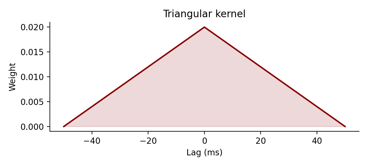
133def triangular_kernel(sigma, dt=1):
134    r"""Return a normalized triangular smoothing kernel.
135
136    Parameters
137    ----------
138    sigma:
139        Target width parameter in ms.
140    dt:
141        Temporal resolution of the target grid in ms.
142
143    Definition
144    ----------
145    Let $a = \sigma \sqrt{6}$. The underlying continuous kernel is
146
147    $$
148    T_\sigma(t) = \frac{\max\left(1 - |t| / a, 0\right)}
149    {\int_{-\infty}^{\infty} \max\left(1 - |u| / a, 0\right)\,du}
150    $$
151
152    and the discrete samples are normalized so that `kernel.sum() * dt = 1`.
153
154    <img src="spiketools_assets/triangular_kernel_example.png"
155         alt="Triangular kernel example"
156         onerror="this.onerror=null;this.src='../spiketools_assets/triangular_kernel_example.png';" />
157
158    Examples
159    --------
160    >>> kernel = triangular_kernel(1.0, dt=1.0)
161    >>> round(kernel.sum(), 3)
162    1.0
163    """
164    half_base = int(pylab.around(sigma * pylab.sqrt(6)))
165    half_kernel = pylab.linspace(0.0, 1.0, half_base + 1)
166    kernel = pylab.append(half_kernel, half_kernel[:-1][::-1])
167    kernel /= dt * kernel.sum()
168    return kernel
Return a normalized triangular smoothing kernel.
Parameters
- sigma:: Target width parameter in ms.
- dt:: Temporal resolution of the target grid in ms.
Definition
Let $a = \sigma \sqrt{6}$. The underlying continuous kernel is
$$ T_\sigma(t) = \frac{\max\left(1 - |t| / a, 0\right)} {\int_{-\infty}^{\infty} \max\left(1 - |u| / a, 0\right)\,du} $$
and the discrete samples are normalized so that kernel.sum() * dt = 1.
Examples
>>> kernel = triangular_kernel(1.0, dt=1.0)
>>> round(kernel.sum(), 3)
1.0
192def rate_warped_analysis(
193    spiketimes,
194    window,
195    step=1.0,
196    tlim=None,
197    rate=None,
198    func=lambda x: x.shape[1] / x[1].max(),
199    kwargs=None,
200    rate_kernel=None,
201    dt=1.0,
202):
203    r"""
204    Apply a function after warping time according to instantaneous rate.
205
206    Parameters
207    ----------
208    spiketimes:
209        Canonical spike representation.
210    window:
211        Window size in warped time. Use `"full"` to analyze the complete warped
212        recording at once.
213    step:
214        Step size in warped time.
215    tlim:
216        Optional `[tmin, tmax]` interval in ms.
217    rate:
218        Optional precomputed `(rate, time)` tuple as returned by
219        `kernel_rate(...)`.
220    func:
221        Statistic to evaluate on the warped spike train.
222    kwargs:
223        Optional keyword arguments forwarded to `func`.
224    rate_kernel:
225        Kernel used when `rate` is not provided.
226    dt:
227        Sampling interval in ms used for the rate estimate.
228
229    Definition
230    ----------
231    The idea is to replace real time $t$ by warped time $\tau(t)$,
232
233    $$
234    \tau(t) = \int_{t_0}^{t} \frac{r(u)}{1000}\,du,
235    $$
236
237    where $r(u)$ is an estimated firing rate in spikes/s. Equal distances on
238    the warped axis therefore correspond to equal expected spike counts. High-
239    rate epochs are stretched, low-rate epochs are compressed, and the chosen
240    statistic is then evaluated on this transformed spike train. If windowed
241    output is requested, the resulting window centers are mapped back to real
242    time before returning.
243
244    Examples
245    --------
246    >>> spikes = pylab.array([[0.0, 3.0, 6.0], [0.0, 0.0, 0.0]])
247    >>> result, warped_duration = rate_warped_analysis(
248    ...     spikes,
249    ...     window="full",
250    ...     func=lambda s: s.shape[1],
251    ...     rate=(pylab.array([[500.0, 500.0, 500.0]]), pylab.array([0.0, 1.0, 2.0])),
252    ...     dt=1.0,
253    ... )
254    >>> int(result), round(float(warped_duration), 3)
255    (3, 1.5)
256    """
257    if kwargs is None:
258        kwargs = {}
259    if rate_kernel is None:
260        rate_kernel = gaussian_kernel(50.0)
261    if rate is None:
262        rate = kernel_rate(spiketimes, rate_kernel, tlim)
263
264    rate, trate = rate
265    rate_tlim = [trate.min(), trate.max() + 1]
266    spiketimes = cut_spiketimes(spiketimes, rate_tlim)
267
268    ot = pylab.cumsum(rate) / 1000.0 * dt
269    w_spiketimes = spiketimes.copy()
270    w_spiketimes[0, :] = time_warp(spiketimes[0, :], trate, ot)
271
272    if window == "full":
273        return func(w_spiketimes, **kwargs), ot.max()
274
275    result, tresult = time_resolved(
276        w_spiketimes, window, func, kwargs, tstep=step
277    )
278    tresult = time_warp(tresult, ot, trate)
279    return result, tresult
Apply a function after warping time according to instantaneous rate.
Parameters
- spiketimes:: Canonical spike representation.
- window:: Window size in warped time. Use
"full"to analyze the complete warped recording at once. - step:: Step size in warped time.
- tlim:: Optional
[tmin, tmax]interval in ms. - rate:: Optional precomputed
(rate, time)tuple as returned bykernel_rate(...). - func:: Statistic to evaluate on the warped spike train.
- kwargs:: Optional keyword arguments forwarded to
func. - rate_kernel:: Kernel used when
rateis not provided. - dt:: Sampling interval in ms used for the rate estimate.
Definition
The idea is to replace real time $t$ by warped time $\tau(t)$,
$$ \tau(t) = \int_{t_0}^{t} \frac{r(u)}{1000}\,du, $$
where $r(u)$ is an estimated firing rate in spikes/s. Equal distances on the warped axis therefore correspond to equal expected spike counts. High- rate epochs are stretched, low-rate epochs are compressed, and the chosen statistic is then evaluated on this transformed spike train. If windowed output is requested, the resulting window centers are mapped back to real time before returning.
Examples
>>> spikes = pylab.array([[0.0, 3.0, 6.0], [0.0, 0.0, 0.0]])
>>> result, warped_duration = rate_warped_analysis(
...     spikes,
...     window="full",
...     func=lambda s: s.shape[1],
...     rate=(pylab.array([[500.0, 500.0, 500.0]]), pylab.array([0.0, 1.0, 2.0])),
...     dt=1.0,
... )
>>> int(result), round(float(warped_duration), 3)
(3, 1.5)
 52def time_resolved(
 53    spiketimes,
 54    window,
 55    func: Callable,
 56    kwargs=None,
 57    tlim: Optional[Sequence[float]] = None,
 58    tstep=1.0,
 59):
 60    r"""
 61    Apply a function to successive windows of a spike train.
 62
 63    Parameters
 64    ----------
 65    spiketimes:
 66        Canonical spike representation.
 67    window:
 68        Window size in ms.
 69    func:
 70        Callable receiving the cropped `spiketimes` of each window.
 71    kwargs:
 72        Optional keyword arguments passed to `func`.
 73    tlim:
 74        Optional analysis interval `[tmin, tmax]` in ms.
 75    tstep:
 76        Window step size in ms.
 77
 78    Returns
 79    -------
 80    tuple[list, np.ndarray]
 81        Function outputs and window-center times.
 82
 83    Definition
 84    ----------
 85    If $S$ denotes the spike train and $f$ the analysis function, then
 86
 87    $$
 88    y_n = f\left(S \cap [t_n, t_n + W)\right),
 89    \qquad
 90    t_n^\mathrm{center} = t_n + \frac{W}{2},
 91    $$
 92
 93    where $W$ is the window width and consecutive windows are offset by
 94    `tstep`.
 95
 96    Examples
 97    --------
 98    >>> spikes = pylab.array([[0.0, 2.0, 4.0], [0.0, 0.0, 0.0]])
 99    >>> values, times = time_resolved(spikes, window=2.0, func=lambda s: s.shape[1], tlim=[0.0, 5.0], tstep=1.0)
100    >>> values
101    [1, 1, 1, 1]
102    >>> times.tolist()
103    [0.5, 1.5, 2.5, 3.5]
104    """
105    if kwargs is None:
106        kwargs = {}
107    if tlim is None:
108        tlim = get_time_limits(spiketimes)
109    cut_spikes = cut_spiketimes(spiketimes, tlim)
110
111    tmin = tlim[0]
112    tmax = tmin + window
113    tcenter = tmin + 0.5 * (tmax - tstep - tmin)
114
115    time = []
116    func_out = []
117    while tmax <= tlim[1]:
118        windowspikes = cut_spiketimes(cut_spikes, [tmin, tmax])
119        time.append(tcenter)
120        func_out.append(func(windowspikes, **kwargs))
121
122        tmin += tstep
123        tmax += tstep
124        tcenter += tstep
125
126    return func_out, pylab.array(time)
Apply a function to successive windows of a spike train.
Parameters
- spiketimes:: Canonical spike representation.
- window:: Window size in ms.
- func:: Callable receiving the cropped
spiketimesof each window. - kwargs:: Optional keyword arguments passed to
func. - tlim:: Optional analysis interval
[tmin, tmax]in ms. - tstep:: Window step size in ms.
Returns
- tuple[list, np.ndarray]: Function outputs and window-center times.
Definition
If $S$ denotes the spike train and $f$ the analysis function, then
$$ y_n = f\left(S \cap [t_n, t_n + W)\right), \qquad t_n^\mathrm{center} = t_n + \frac{W}{2}, $$
where $W$ is the window width and consecutive windows are offset by
tstep.
Examples
>>> spikes = pylab.array([[0.0, 2.0, 4.0], [0.0, 0.0, 0.0]])
>>> values, times = time_resolved(spikes, window=2.0, func=lambda s: s.shape[1], tlim=[0.0, 5.0], tstep=1.0)
>>> values
[1, 1, 1, 1]
>>> times.tolist()
[0.5, 1.5, 2.5, 3.5]
129def time_resolved_new(
130    spiketimes,
131    window,
132    func: Callable,
133    kwargs=None,
134    tlim: Optional[Sequence[float]] = None,
135    tstep=1.0,
136):
137    r"""
138    Windowed evaluation using an intermediate binary representation.
139
140    This variant can be faster for repeated window extraction because the spike
141    train is binned once before the loop.
142
143    Definition
144    ----------
145    This function evaluates the same windowed statistic as `time_resolved(...)`,
146    but it first bins the spike train into a count matrix $B$ and reconstructs
147    each window from the relevant slice:
148
149    Let $k_{n} = \lfloor t_{n} \rfloor$ be the left window index on the binned
150    grid and let $K = \lfloor W \rfloor$ be the corresponding window width in
151    bins. Let $B_{n}$ denote the corresponding slice of the count matrix and let
152    $\mathcal{C}$ denote the conversion from a binary window back to spike
153    times. The statistic is then
154
155    $$
156    y_n = f\left(\mathcal{C}(B_{n})\right).
157    $$
158
159    Examples
160    --------
161    >>> spikes = pylab.array([[0.0, 2.0, 4.0], [0.0, 0.0, 0.0]])
162    >>> values, times = time_resolved_new(spikes, window=2.0, func=lambda s: s.shape[1], tlim=[0.0, 5.0], tstep=1.0)
163    >>> values
164    [1, 1, 1, 1]
165    """
166    if kwargs is None:
167        kwargs = {}
168    if tlim is None:
169        tlim = get_time_limits(spiketimes)
170
171    binary, btime = spiketimes_to_binary(spiketimes, tlim=tlim)
172
173    tmin = tlim[0]
174    tmax = tmin + window
175    tcenter = 0.5 * (tmax + tmin)
176
177    time = []
178    func_out = []
179    while tmax <= tlim[1]:
180        windowspikes = binary_to_spiketimes(
181            binary[:, int(tmin) : int(tmax)], btime[int(tmin) : int(tmax)]
182        )
183        time.append(tcenter)
184        func_out.append(func(windowspikes, **kwargs))
185
186        tmin += tstep
187        tmax += tstep
188        tcenter += tstep
189    return func_out, pylab.array(time)
Windowed evaluation using an intermediate binary representation.
This variant can be faster for repeated window extraction because the spike train is binned once before the loop.
Definition
This function evaluates the same windowed statistic as time_resolved(...),
but it first bins the spike train into a count matrix $B$ and reconstructs
each window from the relevant slice:
Let $k_{n} = \lfloor t_{n} \rfloor$ be the left window index on the binned grid and let $K = \lfloor W \rfloor$ be the corresponding window width in bins. Let $B_{n}$ denote the corresponding slice of the count matrix and let $\mathcal{C}$ denote the conversion from a binary window back to spike times. The statistic is then
$$ y_n = f\left(\mathcal{C}(B_{n})\right). $$
Examples
>>> spikes = pylab.array([[0.0, 2.0, 4.0], [0.0, 0.0, 0.0]])
>>> values, times = time_resolved_new(spikes, window=2.0, func=lambda s: s.shape[1], tlim=[0.0, 5.0], tstep=1.0)
>>> values
[1, 1, 1, 1]
181def cv2(
182    spiketimes,
183    pool=True,
184    return_all=False,
185    bessel_correction=False,
186    minvals=0,
187):
188    r"""Compute the coefficient-of-variation statistic from inter-spike intervals.
189
190    Parameters
191    ----------
192    spiketimes:
193        Canonical spike representation.
194    pool:
195        If `True`, pool intervals across trials or units before computing the
196        statistic. Otherwise compute per row and average.
197    return_all:
198        If `True`, return per-row values instead of their mean.
199    bessel_correction:
200        Use `ddof=1` in the interval variance.
201    minvals:
202        Minimum number of finite intervals required for a per-row value.
203
204    Definition
205    ----------
206    Despite the historical function name, this returns the squared coefficient
207    of variation of the inter-spike intervals $I_n$:
208
209    $$
210    \mathrm{CV}^2 = \frac{\mathrm{Var}[I_n]}{\mathrm{E}[I_n]^2}
211    $$
212
213    Examples
214    --------
215    >>> round(float(cv2(np.array([[0.0, 2.0, 5.0], [0.0, 0.0, 0.0]]))), 3)
216    0.04
217    """
218    if spiketimes.shape[1] < 3:
219        if return_all:
220            return pylab.array([pylab.nan])
221        return pylab.nan
222    ddof = 1 if bessel_correction else 0
223    spikelist = spiketimes_to_list(spiketimes)
224    maxlen = max(len(sl) for sl in spikelist)
225    if maxlen < 3:
226        return pylab.nan
227    spikearray = pylab.zeros((len(spikelist), maxlen)) * pylab.nan
228    spike_counts = []
229    for i, sl in enumerate(spikelist):
230        spikearray[i, : len(sl)] = sl
231        spike_counts.append(len(sl))
232    spike_counts = pylab.array(spike_counts)
233    spikearray = spikearray[spike_counts > 2]
234    intervals = pylab.diff(spikearray, axis=1)
235
236    if pool:
237        var = pylab.nanvar(intervals, ddof=ddof)
238        mean_squared = pylab.nanmean(intervals) ** 2
239        return var / mean_squared
240
241    intervals[pylab.isfinite(intervals).sum(axis=1) < minvals, :] = pylab.nan
242    var = pylab.nanvar(intervals, axis=1, ddof=ddof)
243    mean_squared = pylab.nanmean(intervals, axis=1) ** 2
244    if return_all:
245        return var / mean_squared
246    return pylab.nanmean(var / mean_squared)
Compute the coefficient-of-variation statistic from inter-spike intervals.
Parameters
- spiketimes:: Canonical spike representation.
- pool:: If
True, pool intervals across trials or units before computing the statistic. Otherwise compute per row and average. - return_all:: If
True, return per-row values instead of their mean. - bessel_correction:: Use
ddof=1in the interval variance. - minvals:: Minimum number of finite intervals required for a per-row value.
Definition
Despite the historical function name, this returns the squared coefficient of variation of the inter-spike intervals $I_n$:
$$ \mathrm{CV}^2 = \frac{\mathrm{Var}[I_n]}{\mathrm{E}[I_n]^2} $$
Examples
>>> round(float(cv2(np.array([[0.0, 2.0, 5.0], [0.0, 0.0, 0.0]]))), 3)
0.04
266def cv_two(spiketimes, min_vals=20):
267    r"""Compute the local Cv2 measure from consecutive inter-spike intervals.
268
269    Definition
270    ----------
271    For consecutive inter-spike intervals $I_n$ and $I_{n+1}$, the local Cv2
272    statistic is
273
274    $$
275    \mathrm{Cv2} =
276    \left\langle
277    \frac{2\,|I_{n+1} - I_n|}{I_{n+1} + I_n}
278    \right\rangle_n
279    $$
280
281    where the average is taken across all finite neighboring interval pairs.
282
283    Examples
284    --------
285    >>> round(float(cv_two(np.array([[0.0, 2.0, 5.0, 9.0], [0.0, 0.0, 0.0, 0.0]]), min_vals=2)), 3)
286    0.343
287    """
288    consecutive_isis = _consecutive_intervals(spiketimes)
289    ms = (
290        2
291        * pylab.absolute(consecutive_isis[:, 0] - consecutive_isis[:, 1])
292        / (consecutive_isis[:, 0] + consecutive_isis[:, 1])
293    )
294    if len(ms) >= min_vals:
295        return pylab.mean(ms)
296    return pylab.nan
Compute the local Cv2 measure from consecutive inter-spike intervals.
Definition
For consecutive inter-spike intervals $I_n$ and $I_{n+1}$, the local Cv2 statistic is
$$ \mathrm{Cv2} = \left\langle \frac{2\,|I_{n+1} - I_n|}{I_{n+1} + I_n} \right\rangle_n $$
where the average is taken across all finite neighboring interval pairs.
Examples
>>> round(float(cv_two(np.array([[0.0, 2.0, 5.0, 9.0], [0.0, 0.0, 0.0, 0.0]]), min_vals=2)), 3)
0.343
 99def ff(spiketimes, mintrials=None, tlim=None):
100    r"""Compute the Fano factor across trials or units.
101
102    Parameters
103    ----------
104    spiketimes:
105        Canonical spike representation.
106    mintrials:
107        Optional minimum number of rows required for a valid estimate.
108    tlim:
109        Optional `[tmin, tmax]` counting window in ms.
110
111    Definition
112    ----------
113    If `N` is the spike count in the analysis window, the Fano factor is
114
115    $$
116    \mathrm{FF} = \frac{\mathrm{Var}[N]}{\mathrm{E}[N]}
117    $$
118
119    Examples
120    --------
121    >>> ff(np.array([[0.0, 1.0, 0.0, 1.0], [0.0, 0.0, 1.0, 1.0]]), tlim=[0.0, 2.0])
122    0.0
123    """
124    if tlim is None:
125        tlim = get_time_limits(spiketimes)
126    dt = tlim[1] - tlim[0]
127    binary, _ = spiketimes_to_binary(spiketimes, tlim=tlim, dt=dt)
128    counts = binary.sum(axis=1)
129    if (counts == 0).all():
130        return pylab.nan
131    if mintrials is not None and len(counts) < mintrials:
132        return pylab.nan
133    return counts.var() / counts.mean()
Compute the Fano factor across trials or units.
Parameters
- spiketimes:: Canonical spike representation.
- mintrials:: Optional minimum number of rows required for a valid estimate.
- tlim:: Optional
[tmin, tmax]counting window in ms.
Definition
If N is the spike count in the analysis window, the Fano factor is
$$ \mathrm{FF} = \frac{\mathrm{Var}[N]}{\mathrm{E}[N]} $$
Examples
>>> ff(np.array([[0.0, 1.0, 0.0, 1.0], [0.0, 0.0, 1.0, 1.0]]), tlim=[0.0, 2.0])
0.0
136def kernel_fano(spiketimes, window, dt=1.0, tlim=None, components=False):
137    """Estimate a sliding-window Fano factor from binned spike counts.
138
139    Parameters
140    ----------
141    spiketimes:
142        Canonical spike representation.
143    window:
144        Counting window in ms.
145    dt:
146        Bin width in ms.
147    tlim:
148        Optional analysis interval in ms.
149    components:
150        If `True`, return variance and mean separately instead of their ratio.
151
152    Examples
153    --------
154    >>> fano, time = kernel_fano(
155    ...     np.array([[0.0, 2.0, 0.0, 2.0], [0.0, 0.0, 1.0, 1.0]]),
156    ...     window=2.0,
157    ...     dt=1.0,
158    ...     tlim=[0.0, 4.0],
159    ... )
160    >>> fano.shape, time.shape
161    ((3,), (3,))
162    """
163    if tlim is None:
164        tlim = get_time_limits(spiketimes)
165    if tlim[1] - tlim[0] == window:
166        binary, time = spiketimes_to_binary(spiketimes, tlim=tlim)
167        counts = binary.sum(axis=1)
168        return pylab.array([counts.var() / counts.mean()]), pylab.array(time.mean())
169
170    counts, time = sliding_counts(spiketimes, window, dt, tlim)
171
172    vars_ = counts.var(axis=0)
173    means = counts.mean(axis=0)
174    fano = pylab.zeros_like(vars_) * pylab.nan
175    if components:
176        return vars_, means, time
177    fano[means > 0] = vars_[means > 0] / means[means > 0]
178    return fano, time
Estimate a sliding-window Fano factor from binned spike counts.
Parameters
- spiketimes:: Canonical spike representation.
- window:: Counting window in ms.
- dt:: Bin width in ms.
- tlim:: Optional analysis interval in ms.
- components:: If
True, return variance and mean separately instead of their ratio.
Examples
>>> fano, time = kernel_fano(
...     np.array([[0.0, 2.0, 0.0, 2.0], [0.0, 0.0, 1.0, 1.0]]),
...     window=2.0,
...     dt=1.0,
...     tlim=[0.0, 4.0],
... )
>>> fano.shape, time.shape
((3,), (3,))
299def lv(spiketimes, min_vals=20):
300    r"""Compute the Shinomoto local variation metric.
301
302    Definition
303    ----------
304    Using the same consecutive inter-spike interval notation as `cv_two(...)`,
305    the local variation is
306
307    $$
308    \mathrm{LV} =
309    \left\langle
310    \frac{3\,(I_{n+1} - I_n)^2}{(I_{n+1} + I_n)^2}
311    \right\rangle_n
312    $$
313
314    Unlike $\mathrm{CV}^2$, this statistic is local in time and is therefore
315    less sensitive to slow rate drifts.
316
317    Examples
318    --------
319    >>> round(float(lv(np.array([[0.0, 2.0, 5.0, 9.0], [0.0, 0.0, 0.0, 0.0]]), min_vals=2)), 3)
320    0.091
321    """
322    consecutive_isis = _consecutive_intervals(spiketimes)
323    ms = (
324        3
325        * (consecutive_isis[:, 0] - consecutive_isis[:, 1]) ** 2
326        / (consecutive_isis[:, 0] + consecutive_isis[:, 1]) ** 2
327    )
328    if len(ms) >= min_vals:
329        return pylab.mean(ms)
330    return pylab.nan
Compute the Shinomoto local variation metric.
Definition
Using the same consecutive inter-spike interval notation as cv_two(...),
the local variation is
$$ \mathrm{LV} = \left\langle \frac{3\,(I_{n+1} - I_n)^2}{(I_{n+1} + I_n)^2} \right\rangle_n $$
Unlike $\mathrm{CV}^2$, this statistic is local in time and is therefore less sensitive to slow rate drifts.
Examples
>>> round(float(lv(np.array([[0.0, 2.0, 5.0, 9.0], [0.0, 0.0, 0.0, 0.0]]), min_vals=2)), 3)
0.091
333def time_resolved_cv2(
334    spiketimes,
335    window=None,
336    ot=5.0,
337    tlim=None,
338    pool=False,
339    tstep=1.0,
340    bessel_correction=False,
341    minvals=0,
342    return_all=False,
343):
344    r"""Estimate Cv2 in sliding windows over time.
345
346    Parameters
347    ----------
348    spiketimes:
349        Canonical spike representation.
350    window:
351        Window width in ms. If `None`, it is inferred from the mean ISI.
352    ot:
353        Multiplicative factor used when inferring `window`.
354    tlim:
355        Optional analysis interval in ms.
356    pool:
357        Whether to pool intervals across trials or units.
358    tstep:
359        Window step size in ms.
360    bessel_correction:
361        Use `ddof=1` in the interval variance.
362    minvals:
363        Minimum number of intervals per row.
364    return_all:
365        Return per-row values for each window instead of a single mean.
366
367    Definition
368    ----------
369    For a window of width $W$ starting at $t$, this function computes
370
371    $$
372    \mathrm{CV}^2(t) =
373    \mathrm{CV}^2\left(\{I_n : \text{both spikes of } I_n \in [t, t + W)\}\right)
374    $$
375
376    and reports it at the window center. If `window=None`, the code first
377    estimates a characteristic window from the mean inter-spike interval and
378    the factor `ot`.
379
380    Examples
381    --------
382    >>> values, time = time_resolved_cv2(
383    ...     np.array([[0.0, 2.0, 5.0, 9.0], [0.0, 0.0, 0.0, 0.0]]),
384    ...     window=5.0,
385    ...     tlim=[0.0, 10.0],
386    ...     tstep=2.0,
387    ... )
388    >>> values.shape, time.shape
389    ((3,), (3,))
390    """
391    if tlim is None:
392        tlim = get_time_limits(spiketimes)
393
394    if window is None:
395        spikelist = spiketimes_to_list(spiketimes)
396        isis = [pylab.diff(spikes) for spikes in spikelist]
397        meanisi = [isi.mean() for isi in isis if pylab.isnan(isi.mean()) == False]
398        if meanisi:
399            window = sum(meanisi) / float(len(meanisi)) * ot
400        else:
401            window = tlim[1] - tlim[0]
402
403    time = []
404    cvs = []
405    tmin = tlim[0]
406    tmax = tlim[0] + window
407    order = pylab.argsort(spiketimes[0])
408    ordered_spiketimes = spiketimes[:, order]
409    while tmax < tlim[1]:
410        start_ind = bisect_right(ordered_spiketimes[0], tmin)
411        end_ind = bisect_right(ordered_spiketimes[0], tmax)
412        window_spikes = ordered_spiketimes[:, start_ind:end_ind]
413        cvs.append(
414            cv2(
415                window_spikes,
416                pool,
417                bessel_correction=bessel_correction,
418                minvals=minvals,
419                return_all=return_all,
420            )
421        )
422        time.append(0.5 * (tmin + tmax))
423        tmin += tstep
424        tmax += tstep
425    if return_all:
426        if len(cvs) > 0:
427            maxlen = max(len(cv) for cv in cvs)
428            cvs = [cv.tolist() + [pylab.nan] * (maxlen - len(cv)) for cv in cvs]
429        else:
430            cvs = [[]]
431    return pylab.array(cvs), pylab.array(time)
Estimate Cv2 in sliding windows over time.
Parameters
- spiketimes:: Canonical spike representation.
- window:: Window width in ms. If
None, it is inferred from the mean ISI. - ot:: Multiplicative factor used when inferring
window. - tlim:: Optional analysis interval in ms.
- pool:: Whether to pool intervals across trials or units.
- tstep:: Window step size in ms.
- bessel_correction:: Use
ddof=1in the interval variance. - minvals:: Minimum number of intervals per row.
- return_all:: Return per-row values for each window instead of a single mean.
Definition
For a window of width $W$ starting at $t$, this function computes
$$ \mathrm{CV}^2(t) = \mathrm{CV}^2\left({I_n : \text{both spikes of } I_n \in [t, t + W)}\right) $$
and reports it at the window center. If window=None, the code first
estimates a characteristic window from the mean inter-spike interval and
the factor ot.
Examples
>>> values, time = time_resolved_cv2(
...     np.array([[0.0, 2.0, 5.0, 9.0], [0.0, 0.0, 0.0, 0.0]]),
...     window=5.0,
...     tlim=[0.0, 10.0],
...     tstep=2.0,
... )
>>> values.shape, time.shape
((3,), (3,))
604def time_resolved_cv_two(spiketimes, window=400, tlim=None, min_vals=10, tstep=1):
605    r"""Compute rolling Cv2 using the optional C extension.
606
607    Definition
608    ----------
609    This is the compiled analogue of applying `cv_two(...)` in successive
610    windows. For each window $[t, t + W)$ it collects all finite neighboring
611    interval pairs $(I_n, I_{n+1})$ whose spikes lie inside the window and
612    evaluates
613
614    $$
615    \mathrm{Cv2}(t) =
616    \left\langle
617    \frac{2\,|I_{n+1} - I_n|}{I_{n+1} + I_n}
618    \right\rangle_n
619    $$
620
621    if at least `min_vals` pairs are available. The window is then shifted by
622    `tstep`.
623
624    Notes
625    -----
626    This function requires the optional `Cspiketools` extension module.
627
628    Expected output
629    ---------------
630    Returns `(values, time)` with the same window semantics as
631    `time_resolved_cv2(...)` when the compiled extension is available.
632    """
633    return _time_resolved_cv_two(spiketimes, window, tlim, min_vals, tstep)
Compute rolling Cv2 using the optional C extension.
Definition
This is the compiled analogue of applying cv_two(...) in successive
windows. For each window $[t, t + W)$ it collects all finite neighboring
interval pairs $(I_n, I_{n+1})$ whose spikes lie inside the window and
evaluates
$$ \mathrm{Cv2}(t) = \left\langle \frac{2\,|I_{n+1} - I_n|}{I_{n+1} + I_n} \right\rangle_n $$
if at least min_vals pairs are available. The window is then shifted by
tstep.
Notes
This function requires the optional Cspiketools extension module.
Expected output
Returns (values, time) with the same window semantics as
time_resolved_cv2(...) when the compiled extension is available.
434def time_warped_cv2(
435    spiketimes,
436    window=None,
437    ot=5.0,
438    tstep=1.0,
439    tlim=None,
440    rate=None,
441    kernel_width=50.0,
442    nstd=3.0,
443    pool=True,
444    dt=1.0,
445    inspection_plots=False,
446    kernel_type="gaussian",
447    bessel_correction=False,
448    interpolate=False,
449    minvals=0,
450    return_all=False,
451):
452    """Estimate Cv2 after compensating for slow rate fluctuations by time warping.
453
454    Parameters
455    ----------
456    spiketimes:
457        Canonical spike representation.
458    window:
459        Window width in warped time. If `None`, infer from the mean ISI.
460    ot:
461        Multiplicative factor used for automatic window selection.
462    tstep:
463        Window step size in ms.
464    tlim:
465        Optional `[tmin, tmax]` analysis interval.
466    rate:
467        Optional precomputed `(rate, time)` tuple.
468    kernel_width:
469        Gaussian kernel width in ms when `rate` is not provided.
470    pool:
471        Whether to pool intervals across rows in the Cv2 estimate.
472    dt:
473        Rate-estimation sampling interval in ms.
474    inspection_plots:
475        Plot the forward and backward time-warp mappings for debugging.
476    interpolate:
477        If `True`, interpolate the output back onto a regular time grid.
478    minvals:
479        Minimum number of intervals per row.
480    return_all:
481        Return per-row values for each window instead of a single mean.
482
483    Examples
484    --------
485    >>> values, time = time_warped_cv2(
486    ...     np.array([[0.0, 3.0, 7.0, 12.0], [0.0, 0.0, 0.0, 0.0]]),
487    ...     window=3.0,
488    ...     tlim=[0.0, 13.0],
489    ...     pool=True,
490    ...     dt=1.0,
491    ... )
492    >>> time.ndim
493    1
494    """
495    del nstd  # Unused but kept for API compatibility.
496    del kernel_type  # Unused but kept for API compatibility.
497
498    if tlim is None:
499        tlim = get_time_limits(spiketimes)
500
501    if rate is None:
502        kernel = gaussian_kernel(kernel_width, dt)
503        rate, trate = kernel_rate(spiketimes, kernel, tlim=tlim, dt=dt)
504    else:
505        trate = rate[1]
506        rate = rate[0]
507
508    rate = rate.flatten()
509    rate[rate == 0] = 1e-4
510    notnaninds = pylab.isnan(rate) == False
511    rate = rate[notnaninds]
512    trate = trate[notnaninds]
513
514    tdash = rate_integral(rate, dt)
515    tdash -= tdash.min()
516    tdash /= tdash.max()
517    tdash *= trate.max() - trate.min()
518    tdash += trate.min()
519
520    transformed_spikes = spiketimes.copy().astype(float)
521    transformed_spikes[0, :] = time_warp(transformed_spikes[0, :], trate, tdash)
522
523    if inspection_plots:
524        pylab.figure()
525        pylab.subplot(1, 2, 1)
526        stepsize = max(1, int(spiketimes.shape[1] / 100))
527        for i in list(range(0, spiketimes.shape[1], stepsize)) + [-1]:
528            if pylab.isnan(transformed_spikes[0, i]) or pylab.isnan(spiketimes[0, i]):
529                continue
530            idx_real = int(np.argmin(np.abs(trate - spiketimes[0, i])))
531            idx_warp = int(np.argmin(np.abs(tdash - transformed_spikes[0, i])))
532            pylab.plot(
533                [spiketimes[0, i]] * 2,
534                [0, tdash[idx_real]],
535                "--k",
536                linewidth=0.5,
537            )
538            pylab.plot(
539                [0, trate[idx_warp]],
540                [transformed_spikes[0, i]] * 2,
541                "--k",
542                linewidth=0.5,
543            )
544        pylab.plot(trate, tdash, linewidth=2.0)
545        pylab.xlabel("real time")
546        pylab.ylabel("transformed time")
547        pylab.title("transformation of spiketimes")
548
549    cv2_vals, tcv2 = time_resolved_cv2(
550        transformed_spikes,
551        window,
552        ot,
553        None,
554        pool,
555        tstep,
556        bessel_correction=bessel_correction,
557        minvals=minvals,
558        return_all=return_all,
559    )
560    if inspection_plots:
561        pylab.subplot(1, 2, 2)
562        stepsize = max(1, int(len(tcv2) / 50))
563        tcv22 = time_warp(tcv2, tdash, trate)
564        for i in list(range(0, len(tcv2), stepsize)) + [-1]:
565            idx_warp = int(np.argmin(np.abs(tdash - tcv2[i])))
566            idx_real = int(np.argmin(np.abs(trate - tcv22[i])))
567            pylab.plot(
568                [tcv2[i]] * 2,
569                [0, trate[idx_warp]],
570                "--k",
571                linewidth=0.5,
572            )
573            pylab.plot(
574                [0, tdash[idx_real]],
575                [tcv22[i]] * 2,
576                "--k",
577                linewidth=0.5,
578            )
579        pylab.plot(tdash, trate, linewidth=2)
580        pylab.title("re-transformation of cv2")
581        pylab.xlabel("transformed time")
582        pylab.ylabel("real time")
583
584    tcv2 = time_warp(tcv2, tdash, trate)
585
586    if interpolate:
587        time = pylab.arange(tlim[0], tlim[1], dt)
588        if len(cv2_vals) == 0 or (return_all and cv2_vals.shape[1] == 0):
589            cv2_vals = pylab.zeros_like(time) * pylab.nan
590        else:
591            if return_all:
592                cv2_vals = pylab.array(
593                    [
594                        pylab.interp(time, tcv2, cv2_vals[:, i], left=pylab.nan, right=pylab.nan)
595                        for i in range(cv2_vals.shape[1])
596                    ]
597                )
598            else:
599                cv2_vals = pylab.interp(time, tcv2, cv2_vals, left=pylab.nan, right=pylab.nan)
600        return cv2_vals, time
601    return cv2_vals, tcv2
Estimate Cv2 after compensating for slow rate fluctuations by time warping.
Parameters
- spiketimes:: Canonical spike representation.
- window:: Window width in warped time. If
None, infer from the mean ISI. - ot:: Multiplicative factor used for automatic window selection.
- tstep:: Window step size in ms.
- tlim:: Optional
[tmin, tmax]analysis interval. - rate:: Optional precomputed
(rate, time)tuple. - kernel_width:: Gaussian kernel width in ms when
rateis not provided. - pool:: Whether to pool intervals across rows in the Cv2 estimate.
- dt:: Rate-estimation sampling interval in ms.
- inspection_plots:: Plot the forward and backward time-warp mappings for debugging.
- interpolate:: If
True, interpolate the output back onto a regular time grid. - minvals:: Minimum number of intervals per row.
- return_all:: Return per-row values for each window instead of a single mean.
Examples
>>> values, time = time_warped_cv2(
...     np.array([[0.0, 3.0, 7.0, 12.0], [0.0, 0.0, 0.0, 0.0]]),
...     window=3.0,
...     tlim=[0.0, 13.0],
...     pool=True,
...     dt=1.0,
... )
>>> time.ndim
1
100def resample(vals, time, new_time):
101    """Interpolate a time-resolved signal onto a new time axis.
102
103    Parameters
104    ----------
105    vals:
106        Values sampled on `time`.
107    time:
108        Original sampling points.
109    new_time:
110        Target sampling points.
111
112    Examples
113    --------
114    >>> resample([0.0, 1.0], [0.0, 2.0], [0.0, 1.0, 2.0]).tolist()
115    [0.0, 0.5, 1.0]
116    """
117    if len(vals) > 0:
118        return pylab.interp(new_time, time, vals, right=pylab.nan, left=pylab.nan)
119    return pylab.ones(new_time.shape) * pylab.nan
Interpolate a time-resolved signal onto a new time axis.
Parameters
- vals:: Values sampled on
time. - time:: Original sampling points.
- new_time:: Target sampling points.
Examples
>>> resample([0.0, 1.0], [0.0, 2.0], [0.0, 1.0, 2.0]).tolist()
[0.0, 0.5, 1.0]
60def time_stretch(spiketimes, stretchstart, stretchend, endtime=None):
61    """Stretch trial-wise spike times between two markers to a common duration.
62
63    Parameters
64    ----------
65    spiketimes:
66        Canonical spike representation. The function modifies and returns this
67        array in place.
68    stretchstart:
69        One start time per trial.
70    stretchend:
71        One end time per trial.
72    endtime:
73        Common target end time. Defaults to the mean of `stretchend`.
74
75    Examples
76    --------
77    >>> spikes = pylab.array([[1.0, 3.0, 2.0], [0.0, 0.0, 1.0]])
78    >>> stretched = time_stretch(spikes.copy(), pylab.array([0.0, 0.0]), pylab.array([4.0, 2.0]), endtime=4.0)
79    >>> stretched[0].tolist()
80    [1.0, 3.0, 4.0]
81    """
82    if endtime is None:
83        endtime = stretchend.mean()
84
85    trials = pylab.unique(spiketimes[1, :])
86
87    for i, trial in enumerate(trials):
88        trialmask = spiketimes[1, :] == trial
89        trialspikes = spiketimes[0, trialmask]
90        trialspikes -= stretchstart[i]
91        se = stretchend[i] - stretchstart[i]
92        trialspikes /= se
93        trialspikes *= endtime - stretchstart[i]
94        trialspikes += stretchstart[i]
95        spiketimes[0, trialmask] = trialspikes
96
97    return spiketimes
Stretch trial-wise spike times between two markers to a common duration.
Parameters
- spiketimes:: Canonical spike representation. The function modifies and returns this array in place.
- stretchstart:: One start time per trial.
- stretchend:: One end time per trial.
- endtime:: Common target end time. Defaults to the mean of
stretchend.
Examples
>>> spikes = pylab.array([[1.0, 3.0, 2.0], [0.0, 0.0, 1.0]])
>>> stretched = time_stretch(spikes.copy(), pylab.array([0.0, 0.0]), pylab.array([4.0, 2.0]), endtime=4.0)
>>> stretched[0].tolist()
[1.0, 3.0, 4.0]
35def time_warp(events, told, tnew):
36    """Map event times from one timeline onto another by interpolation.
37
38    Parameters
39    ----------
40    events:
41        Event times to transform.
42    told:
43        Original reference time axis.
44    tnew:
45        New reference axis aligned to `told`.
46
47    Returns
48    -------
49    np.ndarray
50        Warped event times. Values outside the interpolation range become `nan`.
51
52    Examples
53    --------
54    >>> time_warp([0.0, 5.0, 10.0], [0.0, 10.0], [0.0, 20.0]).tolist()
55    [0.0, 10.0, 20.0]
56    """
57    return pylab.interp(events, told, tnew, left=pylab.nan, right=pylab.nan)
Map event times from one timeline onto another by interpolation.
Parameters
- events:: Event times to transform.
- told:: Original reference time axis.
- tnew:: New reference axis aligned to
told.
Returns
- np.ndarray: Warped event times. Values outside the interpolation range become
nan.
Examples
>>> time_warp([0.0, 5.0, 10.0], [0.0, 10.0], [0.0, 20.0]).tolist()
[0.0, 10.0, 20.0]
31def synchrony(spikes, ignore_zero_rows=True):
32    r"""
33    Calculate the Golomb & Hansel (2000) population synchrony measure.
34
35    Parameters
36    ----------
37    spikes:
38        Binned spike matrix with shape `(n_units, n_time_bins)` or a stack of
39        such matrices with trials along the first axis.
40    ignore_zero_rows:
41        If `True`, units with zero spikes are excluded from the statistic.
42
43    Returns
44    -------
45    float
46        Synchrony estimate between `0` and `1` for typical inputs.
47
48    Definition
49    ----------
50    If $x_i(t)$ is the binned activity of unit $i$ and $\langle \cdot \rangle_i$
51    denotes the population average, this implementation returns
52
53    $$
54    \chi =
55    \sqrt{
56    \frac{\mathrm{Var}_t\left[\langle x_i(t) \rangle_i\right]}
57    {\left\langle \mathrm{Var}_t[x_i(t)] \right\rangle_i}
58    }.
59    $$
60
61    Values near `0` indicate largely independent activity, while larger values
62    indicate that the population fluctuates together on the chosen time grid.
63
64    Notes
65    -----
66    This function expects a dense spike-count matrix, not canonical
67    `spiketimes`. Convert first with `spiketimes_to_binary(...)` if needed.
68
69    Examples
70    --------
71    >>> round(float(synchrony(pylab.array([[1, 0, 1], [0, 1, 0]]))), 3)
72    0.0
73    """
74    if len(spikes.shape) > 2:
75        return pylab.array([synchrony(s, ignore_zero_rows) for s in spikes]).mean()
76    if ignore_zero_rows:
77        mask = spikes.sum(axis=1) > 0
78        sync = spikes[mask].mean(axis=0).var() / spikes[mask].var(axis=1).mean()
79    else:
80        sync = spikes.mean(axis=0).var() / spikes.var(axis=1).mean()
81    return sync ** 0.5
Calculate the Golomb & Hansel (2000) population synchrony measure.
Parameters
- spikes:: Binned spike matrix with shape
(n_units, n_time_bins)or a stack of such matrices with trials along the first axis. - ignore_zero_rows:: If
True, units with zero spikes are excluded from the statistic.
Returns
- float: Synchrony estimate between
0and1for typical inputs.
Definition
If $x_i(t)$ is the binned activity of unit $i$ and $\langle \cdot \rangle_i$ denotes the population average, this implementation returns
$$ \chi = \sqrt{ \frac{\mathrm{Var}_t\left[\langle x_i(t) \rangle_i\right]} {\left\langle \mathrm{Var}_t[x_i(t)] \right\rangle_i} }. $$
Values near 0 indicate largely independent activity, while larger values
indicate that the population fluctuates together on the chosen time grid.
Notes
This function expects a dense spike-count matrix, not canonical
spiketimes. Convert first with spiketimes_to_binary(...) if needed.
Examples
>>> round(float(synchrony(pylab.array([[1, 0, 1], [0, 1, 0]]))), 3)
0.0
 28def gamma_spikes(rates, order=[1], tlim=[0.0, 1000.0], dt=0.1):
 29    r"""Generate surrogate spike trains from homogeneous gamma-renewal processes.
 30
 31    Parameters
 32    ----------
 33    rates:
 34        Scalar or per-train firing rates in spikes/s.
 35    order:
 36        Gamma-process shape parameter per train. `1` corresponds to a Poisson
 37        process, values larger than `1` are more regular, and values below `1`
 38        are more bursty.
 39    tlim:
 40        Two-element time interval `[tmin, tmax]` in ms.
 41    dt:
 42        Output quantization step in ms. Generated spike times are rounded to
 43        this grid for backwards compatibility.
 44
 45    Returns
 46    -------
 47    np.ndarray
 48        Canonical `spiketimes` array.
 49
 50    Definition
 51    ----------
 52    For each spike train, consecutive inter-spike intervals are drawn
 53    independently as
 54
 55    $$
 56    I_n \sim \mathrm{Gamma}(k, \theta),
 57    \qquad
 58    k = \mathrm{order},
 59    \qquad
 60    \theta = \frac{1000}{\mathrm{rate}\,k}
 61    $$
 62
 63    so that
 64
 65    $$
 66    \mathrm{E}[I_n] = \frac{1000}{\mathrm{rate}},
 67    \qquad
 68    \mathrm{CV}^2 = \frac{1}{k}.
 69    $$
 70
 71    Examples
 72    --------
 73    >>> np.random.seed(0)
 74    >>> spikes = gamma_spikes([10.0], order=[0.5], tlim=[0.0, 10.0], dt=1.0)
 75    >>> spikes.shape[0]
 76    2
 77    """
 78    rates_arr = np.atleast_1d(np.asarray(rates, dtype=float))
 79    order_arr = np.atleast_1d(np.asarray(order, dtype=float))
 80
 81    if rates_arr.size == 1 and order_arr.size > 1:
 82        rates_arr = np.full(order_arr.shape, rates_arr.item(), dtype=float)
 83    elif order_arr.size == 1 and rates_arr.size > 1:
 84        order_arr = np.full(rates_arr.shape, order_arr.item(), dtype=float)
 85    elif rates_arr.size != order_arr.size:
 86        raise ValueError("`rates` and `order` must have matching lengths or be scalar.")
 87
 88    if np.any(rates_arr <= 0.0):
 89        raise ValueError("All firing rates must be positive.")
 90    if np.any(order_arr <= 0.0):
 91        raise ValueError("All gamma orders must be positive.")
 92
 93    tmin, tmax = float(tlim[0]), float(tlim[1])
 94    if tmax <= tmin:
 95        raise ValueError("`tlim` must satisfy tmax > tmin.")
 96    if dt <= 0.0:
 97        raise ValueError("`dt` must be positive.")
 98
 99    spiketimes = [[], []]
100    for trial_id, (rate_hz, shape) in enumerate(zip(rates_arr, order_arr)):
101        scale_ms = 1000.0 / (rate_hz * shape)
102        t = tmin + np.random.gamma(shape=shape, scale=scale_ms)
103        generated = []
104        while t < tmax:
105            rounded = np.round((t - tmin) / dt) * dt + tmin
106            if rounded < tmax:
107                generated.append(float(rounded))
108            t += np.random.gamma(shape=shape, scale=scale_ms)
109
110        if generated:
111            spiketimes[0].extend(generated)
112            spiketimes[1].extend([float(trial_id)] * len(generated))
113        else:
114            spiketimes[0].append(pylab.nan)
115            spiketimes[1].append(float(trial_id))
116
117    return pylab.array(spiketimes, dtype=float)
Generate surrogate spike trains from homogeneous gamma-renewal processes.
Parameters
- rates:: Scalar or per-train firing rates in spikes/s.
- order:: Gamma-process shape parameter per train.
1corresponds to a Poisson process, values larger than1are more regular, and values below1are more bursty. - tlim:: Two-element time interval
[tmin, tmax]in ms. - dt:: Output quantization step in ms. Generated spike times are rounded to this grid for backwards compatibility.
Returns
- np.ndarray: Canonical
spiketimesarray.
Definition
For each spike train, consecutive inter-spike intervals are drawn independently as
$$ I_n \sim \mathrm{Gamma}(k, \theta), \qquad k = \mathrm{order}, \qquad \theta = \frac{1000}{\mathrm{rate}\,k} $$
so that
$$ \mathrm{E}[I_n] = \frac{1000}{\mathrm{rate}}, \qquad \mathrm{CV}^2 = \frac{1}{k}. $$
Examples
>>> np.random.seed(0)
>>> spikes = gamma_spikes([10.0], order=[0.5], tlim=[0.0, 10.0], dt=1.0)
>>> spikes.shape[0]
2