plotting
Reusable plotting helpers for figures in this repository.
The package provides three main layers:
- spike rasters via
plot_spike_raster(...) - binary-network onset rasters via
plot_binary_raster(...) - shared figure styling via
FontCfg,style_axes(...), and the public palette helpers
Examples
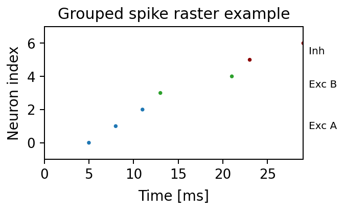
Grouped spike raster example generated from this repository:
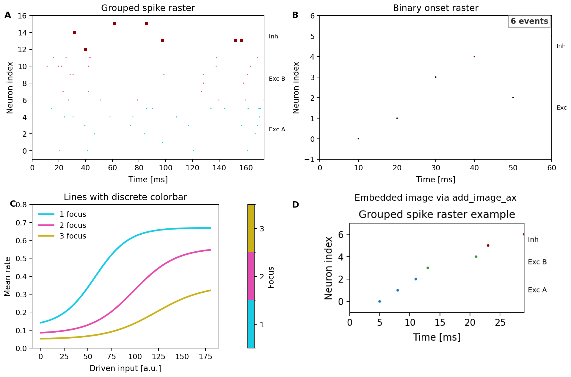
Composite showcase generated from this repository:
Using RasterGroup and RasterLabels explicitly:
import matplotlib.pyplot as plt

from plotting import FontCfg, RasterGroup, RasterLabels, plot_spike_raster, style_axes

groups = [
    RasterGroup("exc_a", ids=range(0, 3), color="#1f77b4", label="Exc A"),
    RasterGroup("exc_b", ids=range(3, 5), color="#2ca02c", label="Exc B"),
    RasterGroup("inh", ids=range(5, 7), color="#8B0000", label="Inh"),
]

fig, ax = plt.subplots(figsize=(4.4, 2.4))
plot_spike_raster(
    ax,
    spike_times_ms=[5, 8, 11, 13, 21, 23, 29],
    spike_ids=[0, 1, 2, 3, 4, 5, 6],
    groups=groups,
    labels=RasterLabels(location="right", kwargs={"fontsize": 8}),
)
ax.set_xlabel("Time [ms]")
ax.set_ylabel("Neuron index")
style_axes(ax, FontCfg().resolve())
fig.tight_layout()
For binary-network traces, use BinaryStateSource together with
plot_binary_raster(...). The generated showcase above includes a full
two-by-two example with grouped spike rasters, binary onset rasters, a discrete
colorbar, and image embedding.
Regenerating docs:
python scripts/generate_api_docs.py
1"""Reusable plotting helpers for figures in this repository. 2 3The package provides three main layers: 4 5- spike rasters via `plot_spike_raster(...)` 6- binary-network onset rasters via `plot_binary_raster(...)` 7- shared figure styling via `FontCfg`, `style_axes(...)`, and the public palette helpers 8 9Examples 10-------- 11 12Grouped spike raster example generated from this repository: 13 14 15 16Composite showcase generated from this repository: 17 18 19 20Using `RasterGroup` and `RasterLabels` explicitly: 21 22```python 23import matplotlib.pyplot as plt 24 25from plotting import FontCfg, RasterGroup, RasterLabels, plot_spike_raster, style_axes 26 27groups = [ 28 RasterGroup("exc_a", ids=range(0, 3), color="#1f77b4", label="Exc A"), 29 RasterGroup("exc_b", ids=range(3, 5), color="#2ca02c", label="Exc B"), 30 RasterGroup("inh", ids=range(5, 7), color="#8B0000", label="Inh"), 31] 32 33fig, ax = plt.subplots(figsize=(4.4, 2.4)) 34plot_spike_raster( 35 ax, 36 spike_times_ms=[5, 8, 11, 13, 21, 23, 29], 37 spike_ids=[0, 1, 2, 3, 4, 5, 6], 38 groups=groups, 39 labels=RasterLabels(location="right", kwargs={"fontsize": 8}), 40) 41ax.set_xlabel("Time [ms]") 42ax.set_ylabel("Neuron index") 43style_axes(ax, FontCfg().resolve()) 44fig.tight_layout() 45``` 46 47For binary-network traces, use `BinaryStateSource` together with 48`plot_binary_raster(...)`. The generated showcase above includes a full 49two-by-two example with grouped spike rasters, binary onset rasters, a discrete 50colorbar, and image embedding. 51 52Regenerating docs: 53 54```bash 55python scripts/generate_api_docs.py 56``` 57""" 58 59from __future__ import annotations 60 61from .spike_raster import RasterGroup, RasterLabels, plot_spike_raster 62from .binary_activity import BinaryStateSource, collect_binary_onset_events, plot_binary_raster 63from .image import add_image_ax 64from .font import ( 65 FontCfg, 66 add_corner_tag, 67 add_panel_label, 68 add_panel_labels_column_left_of_ylabel, 69 style_axes, 70 style_legend, 71 style_colorbar, 72) 73from .time_axis import _time_axis_scale 74from .palette import ( 75 LINE_COLORS, 76 DEFAULT_LINE_COLOR, 77 _cycle_palette, 78 _sample_cmap_colors, 79 _prepare_line_color_map, 80 _prepare_value_color_map, 81 compute_discrete_boundaries, 82 draw_listed_colorbar, 83) 84 85__pdoc__ = { 86 "_time_axis_scale": False, 87 "_cycle_palette": False, 88 "_sample_cmap_colors": False, 89 "_prepare_line_color_map": False, 90 "_prepare_value_color_map": False, 91} 92 93__all__ = [ 94 "RasterGroup", 95 "RasterLabels", 96 "plot_spike_raster", 97 "BinaryStateSource", 98 "collect_binary_onset_events", 99 "plot_binary_raster", 100 "add_image_ax", 101 "FontCfg", 102 "add_corner_tag", 103 "add_panel_label", 104 "add_panel_labels_column_left_of_ylabel", 105 "style_axes", 106 "style_colorbar", 107 "style_legend", 108 "LINE_COLORS", 109 "DEFAULT_LINE_COLOR", 110 "compute_discrete_boundaries", 111 "draw_listed_colorbar", 112]
25@dataclass(frozen=True)
26class RasterGroup:
27    """
28    Definition of a neuron group for spike raster plotting.
29
30    Parameters
31    ----------
32    name:
33        Unique identifier for the group. Used to derive default labels.
34    ids:
35        Specification of neuron membership. May be a slice, range, iterable of ids,
36        NumPy array, or callable returning a boolean mask when applied to neuron ids.
37    color:
38        Matplotlib-compatible color specification for the group's spikes.
39    marker:
40        Marker symbol passed to ``Axes.scatter``.
41    size:
42        Marker size passed to ``Axes.scatter``.
43    label:
44        Optional display label overriding automatic label resolution.
45
46    Examples
47    --------
48    ```python
49    groups = [
50        RasterGroup("exc_a", ids=range(0, 5), color="#1f77b4", label="Exc A"),
51        RasterGroup("inh", ids=range(5, 7), color="#8B0000", label="Inh"),
52    ]
53    ```
54
55    Expected output
56    ---------------
57    Passing `groups` into `plot_spike_raster(...)` draws each group with its own
58    color, marker, and label.
59    """
60
61    name: str
62    ids: GroupIndexer
63    color: str = "black"
64    marker: str = "."
65    size: float = 4.0
66    label: Optional[str] = None
Definition of a neuron group for spike raster plotting.
Parameters
- name:: Unique identifier for the group. Used to derive default labels.
- ids:: Specification of neuron membership. May be a slice, range, iterable of ids, NumPy array, or callable returning a boolean mask when applied to neuron ids.
- color:: Matplotlib-compatible color specification for the group's spikes.
- marker:: Marker symbol passed to
Axes.scatter. - size:: Marker size passed to
Axes.scatter. - label:: Optional display label overriding automatic label resolution.
Examples
groups = [
    RasterGroup("exc_a", ids=range(0, 5), color="#1f77b4", label="Exc A"),
    RasterGroup("inh", ids=range(5, 7), color="#8B0000", label="Inh"),
]
Expected output
Passing groups into plot_spike_raster(...) draws each group with its own
color, marker, and label.
 69@dataclass
 70class RasterLabels:
 71    """
 72    Configuration for annotating neuron groups within a raster plot.
 73
 74    Parameters
 75    ----------
 76    show:
 77        Whether to annotate groups.
 78    mapping:
 79        Explicit mapping of group name -> label text.
 80    excitatory:
 81        Fallback text for groups whose name starts with ``"exc"``.
 82    inhibitory:
 83        Fallback text for groups whose name starts with ``"inh"``.
 84    location:
 85        ``\"right\"`` (default) or ``\"left\"`` indicating where labels should be placed
 86        relative to the plot area.
 87    offset:
 88        Fraction of the x-range used to offset labels from the axis boundary.
 89    kwargs:
 90        Additional keyword arguments forwarded to ``Axes.text``.
 91
 92    Examples
 93    --------
 94    ```python
 95    labels = RasterLabels(
 96        mapping={"exc_a": "Exc A", "inh": "Inh"},
 97        location="right",
 98        kwargs={"fontsize": 9},
 99    )
100    ```
101
102    Expected output
103    ---------------
104    The raster receives one text label per group at the chosen side of the
105    axes.
106    """
107
108    show: bool = True
109    mapping: Mapping[str, str] = field(default_factory=dict)
110    excitatory: Optional[str] = None
111    inhibitory: Optional[str] = None
112    location: str = "right"
113    offset: float = 0.02
114    kwargs: Mapping[str, Any] = field(default_factory=dict)
115
116    def resolve_label(self, group: RasterGroup) -> Optional[str]:
117        if not self.show:
118            return None
119        if group.name in self.mapping:
120            return self.mapping[group.name]
121        if group.label is not None:
122            return group.label
123        gname = group.name.lower()
124        if self.excitatory and gname.startswith("exc"):
125            return self.excitatory
126        if self.inhibitory and gname.startswith("inh"):
127            return self.inhibitory
128        return None
Configuration for annotating neuron groups within a raster plot.
Parameters
- show:: Whether to annotate groups.
- mapping:: Explicit mapping of group name -> label text.
- excitatory:: Fallback text for groups whose name starts with
"exc". - inhibitory:: Fallback text for groups whose name starts with
"inh". - location::
"right"(default) or"left"indicating where labels should be placed relative to the plot area. - offset:: Fraction of the x-range used to offset labels from the axis boundary.
- kwargs:: Additional keyword arguments forwarded to
Axes.text.
Examples
labels = RasterLabels(
    mapping={"exc_a": "Exc A", "inh": "Inh"},
    location="right",
    kwargs={"fontsize": 9},
)
Expected output
The raster receives one text label per group at the chosen side of the axes.
116    def resolve_label(self, group: RasterGroup) -> Optional[str]:
117        if not self.show:
118            return None
119        if group.name in self.mapping:
120            return self.mapping[group.name]
121        if group.label is not None:
122            return group.label
123        gname = group.name.lower()
124        if self.excitatory and gname.startswith("exc"):
125            return self.excitatory
126        if self.inhibitory and gname.startswith("inh"):
127            return self.inhibitory
128        return None
131def plot_spike_raster( 132 ax: plt.Axes, 133 spike_times_ms: Sequence[float], 134 spike_ids: Sequence[int], 135 *, 136 n_exc: Optional[int] = None, 137 n_inh: Optional[int] = None, 138 groups: Optional[Sequence[RasterGroup]] = None, 139 stride: int = 1, 140 t_start: Optional[float] = None, 141 t_end: Optional[float] = None, 142 align_time: Optional[float] = None, 143 time_reference: str = "absolute", 144 reference_time: Optional[float] = None, 145 marker: str = ".", 146 marker_size: float = 4.0, 147 exc_color: str = "black", 148 inh_color: str = "#8B0000", 149 labels: Optional[RasterLabels] = None, 150) -> plt.Axes: 151 """ 152 Plot a configurable spike raster on *ax*. 153 154 Parameters 155 ---------- 156 ax: 157 Target Matplotlib axes. 158 spike_times_ms, spike_ids: 159 1-D sequences of spike times (ms) and corresponding neuron ids. 160 n_exc, n_inh: 161 Sizes of excitatory and inhibitory populations used when *groups* is not provided. 162 groups: 163 Optional explicit group definitions overriding *n_exc* / *n_inh*. 164 stride: 165 Keep every ``stride``-th neuron id (e.g., ``stride=10`` shows every 10th neuron). 166 t_start, t_end: 167 Optional temporal window (after alignment) to display. 168 align_time: 169 Time (ms) subtracted from all spike times prior to plotting. 170 time_reference: 171 Either ``\"absolute\"`` (default) or ``\"relative\"``. When ``\"relative\"`` and 172 *reference_time* is ``None``, the minimum time after alignment is used as reference. 173 reference_time: 174 Time (ms) used as reference when ``time_reference=\"relative\"``. 175 marker, marker_size: 176 Defaults for marker appearance when *groups* is not provided. 177 exc_color, inh_color: 178 Default colors for excitatory/inhibitory groups. 179 labels: 180 Optional :class:`RasterLabels` controlling group annotations. 181 182 Examples 183 -------- 184 ```python 185 fig, ax = plt.subplots(figsize=(4, 2)) 186 groups = [ 187 RasterGroup("exc_a", ids=range(0, 3), color="#1f77b4", label="Exc A"), 188 RasterGroup("exc_b", ids=range(3, 5), color="#2ca02c", label="Exc B"), 189 RasterGroup("inh", ids=range(5, 7), color="#8B0000", label="Inh"), 190 ] 191 plot_spike_raster( 192 ax, 193 spike_times_ms=[5, 8, 11, 13, 21, 23, 29], 194 spike_ids=[0, 1, 2, 3, 4, 5, 6], 195 groups=groups, 196 labels=RasterLabels(location="right", kwargs={"fontsize": 8}), 197 ) 198 ``` 199 200 Expected output 201 --------------- 202 The axes contains one grouped raster with group-specific colors and three 203 group labels at the right margin. 204 205  206 """ 207 times = np.asarray(spike_times_ms, dtype=float) 208 neuron_ids = np.asarray(spike_ids, dtype=int) 209 if times.shape != neuron_ids.shape: 210 raise ValueError("spike_times_ms and spike_ids must have matching shapes.") 211 212 if align_time is not None: 213 times = times - float(align_time) 214 215 time_reference = time_reference.lower() 216 if time_reference not in {"absolute", "relative"}: 217 raise ValueError("time_reference must be 'absolute' or 'relative'.") 218 if time_reference == "relative": 219 ref = reference_time 220 if ref is None: 221 ref = times.min() if times.size else 0.0 222 times = times - float(ref) 223 224 # Temporal selection 225 mask = np.ones(times.shape, dtype=bool) 226 if t_start is not None: 227 mask &= times >= float(t_start) 228 if t_end is not None: 229 mask &= times <= float(t_end) 230 231 # Stride selection 232 stride = max(int(stride), 1) 233 if stride > 1: 234 mask &= (neuron_ids % stride) == 0 235 236 times = times[mask] 237 neuron_ids = neuron_ids[mask] 238 239 resolved_groups = _resolve_groups( 240 groups=groups, 241 n_exc=n_exc, 242 n_inh=n_inh, 243 marker=marker, 244 marker_size=marker_size, 245 exc_color=exc_color, 246 inh_color=inh_color, 247 ) 248 249 for group in resolved_groups: 250 group_mask = _evaluate_group_mask(group.ids, neuron_ids) 251 if not np.any(group_mask): 252 continue 253 ax.scatter( 254 times[group_mask], 255 neuron_ids[group_mask], 256 s=float(group.size) ** 2, 257 c=group.color, 258 marker=group.marker, 259 linewidths=0, 260 edgecolors="none", 261 ) 262 263 # Limits 264 if times.size: 265 xmin = 0.0 if t_start is None else float(t_start) 266 xmax = float(times.max() if t_end is None else t_end) 267 if t_start is not None: 268 xmin = float(t_start) 269 if t_end is not None: 270 xmax = float(t_end) 271 if xmin == xmax: 272 xmax = xmin + 1.0 273 ax.set_xlim(xmin, xmax) 274 else: 275 xmin = float(t_start if t_start is not None else 0.0) 276 xmax = float(t_end if t_end is not None else xmin + 1.0) 277 if xmin == xmax: 278 xmax = xmin + 1.0 279 ax.set_xlim(xmin, xmax) 280 281 if neuron_ids.size: 282 ymin = neuron_ids.min() 283 ymax = neuron_ids.max() 284 else: 285 ymin, ymax = _group_global_bounds(resolved_groups) 286 if ymin == ymax: 287 ymax = ymin + 1 288 padding = max(1, int((ymax - ymin) * 0.02)) 289 ax.set_ylim(ymin - padding, ymax + padding) 290 291 if labels is not None and labels.show: 292 _apply_group_labels(ax, resolved_groups, labels) 293 294 return ax
Plot a configurable spike raster on ax.
Parameters
- ax:: Target Matplotlib axes.
- spike_times_ms, spike_ids:: 1-D sequences of spike times (ms) and corresponding neuron ids.
- n_exc, n_inh:: Sizes of excitatory and inhibitory populations used when groups is not provided.
- groups:: Optional explicit group definitions overriding n_exc / n_inh.
- stride:: Keep every
stride-th neuron id (e.g.,stride=10shows every 10th neuron). - t_start, t_end:: Optional temporal window (after alignment) to display.
- align_time:: Time (ms) subtracted from all spike times prior to plotting.
- time_reference:: Either
"absolute"(default) or"relative". When"relative"and reference_time isNone, the minimum time after alignment is used as reference. - reference_time:: Time (ms) used as reference when
time_reference="relative". - marker, marker_size:: Defaults for marker appearance when groups is not provided.
- exc_color, inh_color:: Default colors for excitatory/inhibitory groups.
- labels:: Optional
RasterLabelscontrolling group annotations.
Examples
fig, ax = plt.subplots(figsize=(4, 2))
groups = [
    RasterGroup("exc_a", ids=range(0, 3), color="#1f77b4", label="Exc A"),
    RasterGroup("exc_b", ids=range(3, 5), color="#2ca02c", label="Exc B"),
    RasterGroup("inh", ids=range(5, 7), color="#8B0000", label="Inh"),
]
plot_spike_raster(
    ax,
    spike_times_ms=[5, 8, 11, 13, 21, 23, 29],
    spike_ids=[0, 1, 2, 3, 4, 5, 6],
    groups=groups,
    labels=RasterLabels(location="right", kwargs={"fontsize": 8}),
)
Expected output
The axes contains one grouped raster with group-specific colors and three group labels at the right margin.
 27@dataclass
 28class BinaryStateSource:
 29    """Describe how binary neuron states are provided for raster plotting.
 30
 31    Parameters
 32    ----------
 33    inline_states:
 34        Optional in-memory state matrix with shape `(steps, neurons)`.
 35    chunk_files:
 36        Optional paths to `.npy` or `.npz` chunks storing state matrices.
 37    neuron_count:
 38        Total number of neurons represented by the source.
 39    update_log, delta_log:
 40        Optional diff-log representation where each column corresponds to a
 41        simulation step.
 42    initial_state:
 43        Optional initial state for diff-log based sources.
 44
 45    Examples
 46    --------
 47    Wrap an in-memory state matrix:
 48
 49    >>> states = np.array([[0, 1], [1, 1], [1, 0]], dtype=np.uint8)
 50    >>> source = BinaryStateSource.from_array(states)
 51    >>> source.neuron_count
 52    2
 53
 54    Wrap diff logs directly:
 55
 56    >>> updates = np.array([[0, 1], [1, 0]], dtype=np.uint16)
 57    >>> deltas = np.array([[1, -1], [0, 1]], dtype=np.int8)
 58    >>> source = BinaryStateSource.from_diff_logs(updates, deltas, neuron_count=2)
 59    >>> source.update_log.shape
 60    (2, 2)
 61    """
 62
 63    inline_states: Optional[np.ndarray] = None
 64    chunk_files: Sequence[Path] = field(default_factory=tuple)
 65    neuron_count: int = 0
 66    update_log: Optional[np.ndarray] = None
 67    delta_log: Optional[np.ndarray] = None
 68    initial_state: Optional[np.ndarray] = None
 69
 70    def iter_chunks(self) -> Iterator[np.ndarray]:
 71        """Yield state chunks with shape `(steps, neurons)`."""
 72        if self.inline_states is not None and self.inline_states.size:
 73            yield np.asarray(self.inline_states, dtype=np.uint8)
 74            return
 75        for entry in self.chunk_files:
 76            path = Path(entry)
 77            if not path.exists():
 78                continue
 79            data = np.load(path, allow_pickle=False, mmap_mode="r")
 80            yield np.asarray(data, dtype=np.uint8)
 81
 82    @classmethod
 83    def from_array(cls, states: Union[np.ndarray, Iterable[Sequence[int]]]) -> "BinaryStateSource":
 84        """Convenience helper for wrapping an in-memory state matrix.
 85
 86        Examples
 87        --------
 88        >>> source = BinaryStateSource.from_array([[0, 1], [1, 1]])
 89        >>> source.neuron_count
 90        2
 91        """
 92        array = np.asarray(states)
 93        neuron_count = int(array.shape[1]) if array.ndim == 2 else 0
 94        return cls(inline_states=array, chunk_files=tuple(), neuron_count=neuron_count)
 95
 96    @classmethod
 97    def from_diff_logs(
 98        cls,
 99        updates: np.ndarray,
100        deltas: np.ndarray,
101        *,
102        neuron_count: int,
103        initial_state: Optional[np.ndarray] = None,
104    ) -> "BinaryStateSource":
105        """Construct a source from diff-log traces.
106
107        Examples
108        --------
109        >>> source = BinaryStateSource.from_diff_logs(
110        ...     np.array([[0, 1]], dtype=np.uint16),
111        ...     np.array([[1, -1]], dtype=np.int8),
112        ...     neuron_count=2,
113        ... )
114        >>> source.neuron_count
115        2
116        """
117        update_arr = np.asarray(updates, dtype=np.uint16)
118        delta_arr = np.asarray(deltas, dtype=np.int8)
119        init_state = None
120        if initial_state is not None:
121            init_state = np.asarray(initial_state, dtype=np.uint8)
122        return cls(
123            inline_states=None,
124            chunk_files=tuple(),
125            neuron_count=int(neuron_count),
126            update_log=update_arr,
127            delta_log=delta_arr,
128            initial_state=init_state,
129        )
Describe how binary neuron states are provided for raster plotting.
Parameters
- inline_states:: Optional in-memory state matrix with shape
(steps, neurons). - chunk_files:: Optional paths to
.npyor.npzchunks storing state matrices. - neuron_count:: Total number of neurons represented by the source.
- update_log, delta_log:: Optional diff-log representation where each column corresponds to a simulation step.
- initial_state:: Optional initial state for diff-log based sources.
Examples
Wrap an in-memory state matrix:
>>> states = np.array([[0, 1], [1, 1], [1, 0]], dtype=np.uint8)
>>> source = BinaryStateSource.from_array(states)
>>> source.neuron_count
2
Wrap diff logs directly:
>>> updates = np.array([[0, 1], [1, 0]], dtype=np.uint16)
>>> deltas = np.array([[1, -1], [0, 1]], dtype=np.int8)
>>> source = BinaryStateSource.from_diff_logs(updates, deltas, neuron_count=2)
>>> source.update_log.shape
(2, 2)
70    def iter_chunks(self) -> Iterator[np.ndarray]:
71        """Yield state chunks with shape `(steps, neurons)`."""
72        if self.inline_states is not None and self.inline_states.size:
73            yield np.asarray(self.inline_states, dtype=np.uint8)
74            return
75        for entry in self.chunk_files:
76            path = Path(entry)
77            if not path.exists():
78                continue
79            data = np.load(path, allow_pickle=False, mmap_mode="r")
80            yield np.asarray(data, dtype=np.uint8)
Yield state chunks with shape (steps, neurons).
82    @classmethod
83    def from_array(cls, states: Union[np.ndarray, Iterable[Sequence[int]]]) -> "BinaryStateSource":
84        """Convenience helper for wrapping an in-memory state matrix.
85
86        Examples
87        --------
88        >>> source = BinaryStateSource.from_array([[0, 1], [1, 1]])
89        >>> source.neuron_count
90        2
91        """
92        array = np.asarray(states)
93        neuron_count = int(array.shape[1]) if array.ndim == 2 else 0
94        return cls(inline_states=array, chunk_files=tuple(), neuron_count=neuron_count)
Convenience helper for wrapping an in-memory state matrix.
Examples
>>> source = BinaryStateSource.from_array([[0, 1], [1, 1]])
>>> source.neuron_count
2
 96    @classmethod
 97    def from_diff_logs(
 98        cls,
 99        updates: np.ndarray,
100        deltas: np.ndarray,
101        *,
102        neuron_count: int,
103        initial_state: Optional[np.ndarray] = None,
104    ) -> "BinaryStateSource":
105        """Construct a source from diff-log traces.
106
107        Examples
108        --------
109        >>> source = BinaryStateSource.from_diff_logs(
110        ...     np.array([[0, 1]], dtype=np.uint16),
111        ...     np.array([[1, -1]], dtype=np.int8),
112        ...     neuron_count=2,
113        ... )
114        >>> source.neuron_count
115        2
116        """
117        update_arr = np.asarray(updates, dtype=np.uint16)
118        delta_arr = np.asarray(deltas, dtype=np.int8)
119        init_state = None
120        if initial_state is not None:
121            init_state = np.asarray(initial_state, dtype=np.uint8)
122        return cls(
123            inline_states=None,
124            chunk_files=tuple(),
125            neuron_count=int(neuron_count),
126            update_log=update_arr,
127            delta_log=delta_arr,
128            initial_state=init_state,
129        )
Construct a source from diff-log traces.
Examples
>>> source = BinaryStateSource.from_diff_logs(
...     np.array([[0, 1]], dtype=np.uint16),
...     np.array([[1, -1]], dtype=np.int8),
...     neuron_count=2,
... )
>>> source.neuron_count
2
132def collect_binary_onset_events(
133    state_source: BinaryStateSource,
134    sample_interval: int,
135    *,
136    window: Optional[Tuple[float, float]] = None,
137) -> tuple[np.ndarray, np.ndarray]:
138    """Collect onset events from a binary state stream.
139
140    Parameters
141    ----------
142    state_source:
143        Binary state source, either as full states or diff logs.
144    sample_interval:
145        Time step between successive recorded samples.
146    window:
147        Optional `(start, end)` filter in the same units as `sample_interval`.
148
149    Returns
150    -------
151    tuple[np.ndarray, np.ndarray]
152        Event times and neuron ids suitable for `plot_spike_raster(...)`.
153
154    Examples
155    --------
156    >>> source = BinaryStateSource.from_array(np.array([[0, 0], [1, 0], [1, 1]], dtype=np.uint8))
157    >>> times, ids = collect_binary_onset_events(source, sample_interval=5)
158    >>> times.tolist()
159    [5.0, 10.0]
160    >>> ids.tolist()
161    [0, 1]
162    """
163    sample_interval = max(1, int(sample_interval))
164    window_start = float(window[0]) if window else None
165    window_end = float(window[1]) if window else None
166    if state_source.update_log is not None and state_source.delta_log is not None:
167        return _collect_from_diff_log(state_source, sample_interval, window=window)
168    times: list[np.ndarray] = []
169    neurons: list[np.ndarray] = []
170    prev_state: Optional[np.ndarray] = None
171    sample_index = 0
172    for chunk in state_source.iter_chunks():
173        block = np.asarray(chunk, dtype=np.uint8)
174        if block.ndim != 2 or block.shape[0] == 0:
175            continue
176        for row in block:
177            sample_index += 1
178            if prev_state is None:
179                prev_state = row.copy()
180                continue
181            transitions = (prev_state == 0) & (row == 1)
182            transition_time = (sample_index - 1) * sample_interval
183            prev_state = row.copy()
184            if window_end is not None and transition_time > window_end:
185                return _finalize(times, neurons)
186            if not transitions.any():
187                continue
188            if window_start is not None and transition_time < window_start:
189                continue
190            idx = np.flatnonzero(transitions)
191            if idx.size == 0:
192                continue
193            times.append(np.full(idx.size, transition_time, dtype=np.float64))
194            neurons.append(idx.astype(np.int64))
195    return _finalize(times, neurons)
Collect onset events from a binary state stream.
Parameters
- state_source:: Binary state source, either as full states or diff logs.
- sample_interval:: Time step between successive recorded samples.
- window:: Optional
(start, end)filter in the same units assample_interval.
Returns
- tuple[np.ndarray, np.ndarray]: Event times and neuron ids suitable for
plot_spike_raster(...).
Examples
>>> source = BinaryStateSource.from_array(np.array([[0, 0], [1, 0], [1, 1]], dtype=np.uint8))
>>> times, ids = collect_binary_onset_events(source, sample_interval=5)
>>> times.tolist()
[5.0, 10.0]
>>> ids.tolist()
[0, 1]
198def plot_binary_raster( 199 ax: Axes, 200 *, 201 state_source: BinaryStateSource, 202 sample_interval: int, 203 n_exc: int, 204 n_inh: Optional[int] = None, 205 total_neurons: Optional[int] = None, 206 window: Optional[Tuple[float, float]] = None, 207 time_scale: float = 1.0, 208 stride: int = 1, 209 labels: Optional[RasterLabels] = None, 210 groups: Optional[Sequence[RasterGroup]] = None, 211 marker: str = ".", 212 marker_size: float = 4.0, 213 empty_text: str = "No neuron onset events", 214 **raster_kwargs, 215) -> tuple[np.ndarray, np.ndarray]: 216 """ 217 Plot a binary-network onset raster. 218 219 The function first extracts onset events from the provided binary state 220 source and then forwards those events to `plot_spike_raster(...)`. 221 222 Examples 223 -------- 224 ```python 225 fig, ax = plt.subplots(figsize=(4, 2)) 226 source = BinaryStateSource.from_array( 227 np.array([[0, 0], [1, 0], [1, 1], [0, 1]], dtype=np.uint8) 228 ) 229 times, ids = plot_binary_raster( 230 ax, 231 state_source=source, 232 sample_interval=10, 233 n_exc=1, 234 n_inh=1, 235 ) 236 ``` 237 238 Expected output 239 --------------- 240 `times` is `array([10., 20.])` and `ids` is `array([0, 1])`. The axes 241 shows two onset markers at those coordinates. 242 243 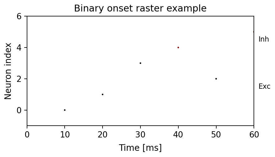 244 """ 245 events = collect_binary_onset_events(state_source, sample_interval, window=window) 246 spike_times, spike_ids = events 247 if spike_times.size == 0 or spike_ids.size == 0: 248 ax.text(0.5, 0.5, empty_text, ha="center", va="center", transform=ax.transAxes) 249 ax.set_axis_off() 250 return events 251 safe_scale = time_scale if time_scale > 0 else 1.0 252 scaled_times = spike_times / safe_scale 253 t_start = (window[0] / safe_scale) if window else None 254 t_end = (window[1] / safe_scale) if window else None 255 256 total = total_neurons or state_source.neuron_count or 0 257 n_exc = max(0, int(n_exc)) 258 if n_inh is None: 259 n_inh = max(0, total - n_exc) 260 n_inh = max(0, int(n_inh)) 261 262 plot_spike_raster( 263 ax=ax, 264 spike_times_ms=scaled_times, 265 spike_ids=spike_ids, 266 n_exc=n_exc, 267 n_inh=n_inh, 268 groups=groups, 269 stride=max(1, int(stride)), 270 t_start=t_start, 271 t_end=t_end, 272 marker=marker, 273 marker_size=marker_size, 274 labels=labels, 275 **raster_kwargs, 276 ) 277 if t_start is not None or t_end is not None: 278 xmin = t_start if t_start is not None else ax.get_xlim()[0] 279 xmax = t_end if t_end is not None else ax.get_xlim()[1] 280 if xmin == xmax: 281 xmax = xmin + 1.0 282 ax.set_xlim(xmin, xmax) 283 return events
Plot a binary-network onset raster.
The function first extracts onset events from the provided binary state
source and then forwards those events to plot_spike_raster(...).
Examples
fig, ax = plt.subplots(figsize=(4, 2))
source = BinaryStateSource.from_array(
    np.array([[0, 0], [1, 0], [1, 1], [0, 1]], dtype=np.uint8)
)
times, ids = plot_binary_raster(
    ax,
    state_source=source,
    sample_interval=10,
    n_exc=1,
    n_inh=1,
)
Expected output
times is array([10., 20.]) and ids is array([0, 1]). The axes
shows two onset markers at those coordinates.

34def add_image_ax(ax, path, label=None, fc: Optional[FontCfg]=None, *, pdf_page: int = 0, pdf_zoom: float = 2.0): 35 """Render an image into an axes and optionally add a panel label. 36 37 Parameters 38 ---------- 39 ax: 40 Target Matplotlib axes. 41 path: 42 Image or PDF path. 43 label: 44 Optional panel label placed near the upper-left corner. 45 fc: 46 Optional `FontCfg` used for the label size. 47 pdf_page, pdf_zoom: 48 PDF rendering options used when `path` points to a PDF. 49 50 Examples 51 -------- 52 ```python 53 fig, ax = plt.subplots(figsize=(3, 2)) 54 add_image_ax(ax, "docs/plotting_assets/spike_raster_example.png", label="A") 55 ``` 56 57 Expected output 58 --------------- 59 The axes displays the image and, when `label` is provided, a bold panel 60 label is drawn near the upper-left corner. 61 62 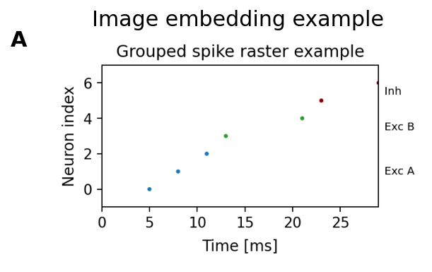 63 """ 64 ax.axis('off') 65 try: 66 img = _imread_any(path, pdf_page=pdf_page, pdf_zoom=pdf_zoom) 67 h, w = img.shape[0], img.shape[1] 68 ax.imshow(img) 69 ax.set_box_aspect(h / w if w else 1) 70 except FileNotFoundError: 71 ax.text(0.5, 0.5, f"Missing image:\n{path}", ha='center', va='center', fontsize=10) 72 ax.set_box_aspect(1) 73 except Exception as e: 74 ax.text(0.5, 0.5, f"Error loading:\n{os.path.basename(path)}\n{e}", ha='center', va='center', fontsize=10) 75 ax.set_box_aspect(1) 76 if label: 77 label_cfg = fc if fc is not None else FontCfg().resolve() 78 add_panel_label(ax, label, label_cfg) 79 return ax
Render an image into an axes and optionally add a panel label.
Parameters
- ax:: Target Matplotlib axes.
- path:: Image or PDF path.
- label:: Optional panel label placed near the upper-left corner.
- fc:: Optional
FontCfgused for the label size. - pdf_page, pdf_zoom:: PDF rendering options used when
pathpoints to a PDF.
Examples
fig, ax = plt.subplots(figsize=(3, 2))
add_image_ax(ax, "docs/plotting_assets/spike_raster_example.png", label="A")
Expected output
The axes displays the image and, when label is provided, a bold panel
label is drawn near the upper-left corner.

20@dataclass
21class FontCfg:
22    """Font-size configuration shared across multi-panel figures.
23
24    Call `resolve()` once after construction to derive unset sizes from the
25    `base` and `scale` values.
26
27    Examples
28    --------
29    >>> cfg = FontCfg(base=10.0, scale=1.2).resolve()
30    >>> round(cfg.label, 1), round(cfg.letter, 1)
31    (12.0, 13.2)
32    """
33    base: float = 12.0
34    scale: float = 1.4
35    title: float = None
36    label: float = None
37    tick: float = None
38    legend: float = None
39    panel: float = None
40    labelpad: float = 6.0
41    letter: float = None          # NEW: subplot letter size
42
43    def resolve(self):
44        """Fill unset size fields from the base configuration."""
45        if self.title  is None: self.title  = self.base * self.scale * 1.20
46        if self.label  is None: self.label  = self.base * self.scale * 1.00
47        if self.tick   is None: self.tick   = self.base * self.scale * 0.95
48        if self.legend is None: self.legend = self.base * self.scale * 0.95
49        if self.panel  is None: self.panel  = self.base * self.scale * 0.95
50        if self.letter is None: self.letter = self.base * self.scale * 1.10
51        return self
Font-size configuration shared across multi-panel figures.
Call resolve() once after construction to derive unset sizes from the
base and scale values.
Examples
>>> cfg = FontCfg(base=10.0, scale=1.2).resolve()
>>> round(cfg.label, 1), round(cfg.letter, 1)
(12.0, 13.2)
43    def resolve(self):
44        """Fill unset size fields from the base configuration."""
45        if self.title  is None: self.title  = self.base * self.scale * 1.20
46        if self.label  is None: self.label  = self.base * self.scale * 1.00
47        if self.tick   is None: self.tick   = self.base * self.scale * 0.95
48        if self.legend is None: self.legend = self.base * self.scale * 0.95
49        if self.panel  is None: self.panel  = self.base * self.scale * 0.95
50        if self.letter is None: self.letter = self.base * self.scale * 1.10
51        return self
Fill unset size fields from the base configuration.
54def add_corner_tag(ax, text, color, fc: FontCfg, *, x=0.985, y=0.985): 55 """Add a boxed annotation tag in the upper-right corner of an axes. 56 57 Expected output 58 --------------- 59 The axes receives one bold text box near its upper-right corner. 60 61 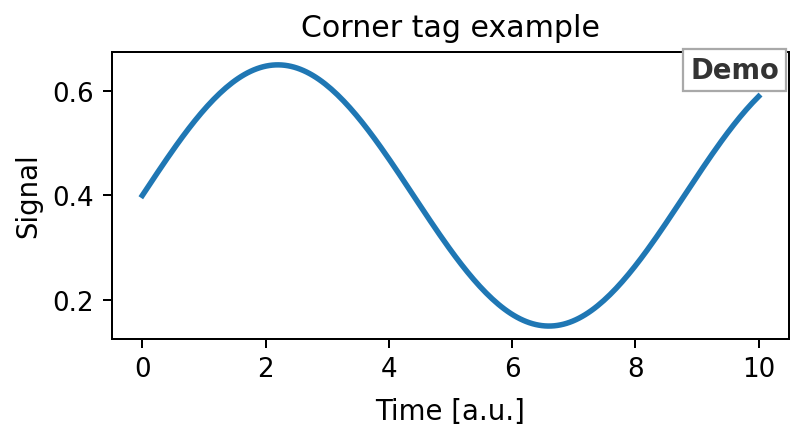 62 """ 63 ax.text( 64 x, y, text, 65 transform=ax.transAxes, 66 ha="right", va="top", 67 fontsize=fc.label, fontweight="bold", color=color, 68 bbox=dict( 69 facecolor="white", 70 edgecolor="darkgrey", 71 linewidth=0.9, 72 boxstyle="square,pad=0.25" 73 ), 74 zorder=10, 75 clip_on=False 76 )
Add a boxed annotation tag in the upper-right corner of an axes.
Expected output
The axes receives one bold text box near its upper-right corner.

78def add_panel_label(ax, text, fc: FontCfg, *, x=-0.12, y=1.03): 79 """Add a bold panel label in axes coordinates. 80 81 Expected output 82 --------------- 83 One bold label appears slightly above and left of the axes, matching the 84 figure panel style used across this repository. 85 86 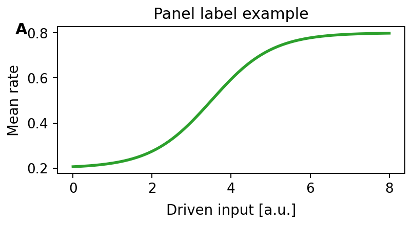 87 """ 88 ax.text(x, y, text, transform=ax.transAxes, 89 ha="left", va="top", fontsize=fc.letter, fontweight="bold", clip_on=False)
Add a bold panel label in axes coordinates.
Expected output
One bold label appears slightly above and left of the axes, matching the figure panel style used across this repository.

90def add_panel_labels_column_left_of_ylabel( 91 axs: List[plt.Axes], 92 texts: List[str], 93 fc: FontCfg, 94 *, 95 pad_pts: float = 6.0, # how far left of the y-label/axes edge (in points) 96 y_axes: float = 0.99 # vertical position within each axes (axes coords) 97): 98 """Place panel labels (texts) in a vertical column left of the y-labels. 99 100 Alignment is computed in figure coordinates from the left-most of: 101 - the y-label bbox (if present), else 102 - the axes bbox (if no y-label). 103 104 Expected output 105 --------------- 106 Each axes receives one label, and all labels are aligned in a shared 107 vertical column left of the y-axis labels. 108 109 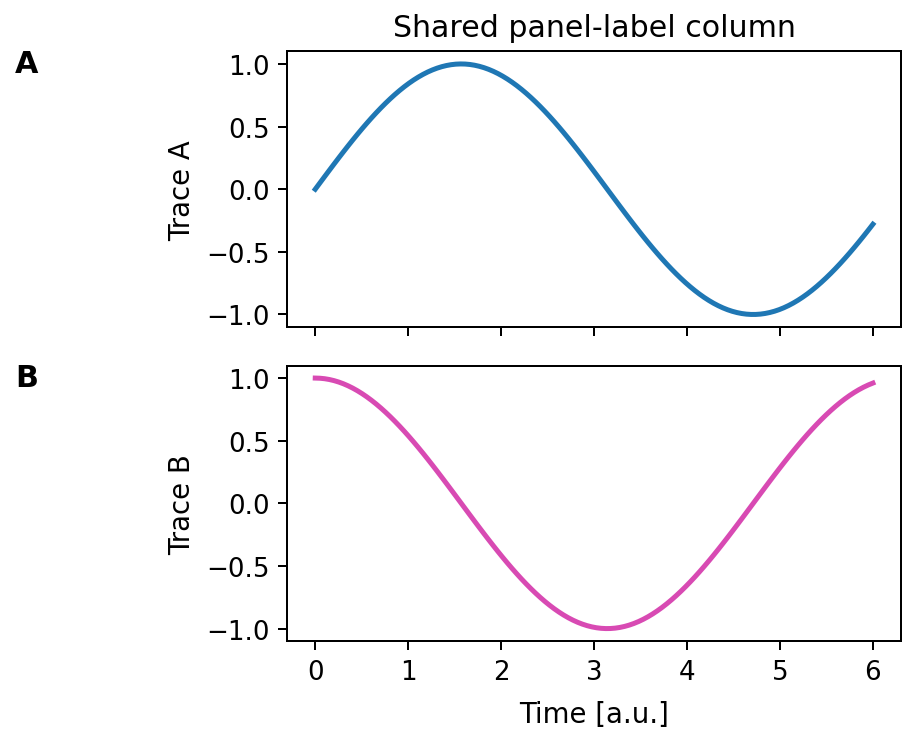 110 """ 111 if not axs: 112 return 113 fig = axs[0].figure 114 115 # Ensure we have a renderer (positions are known) 116 fig.canvas.draw() 117 renderer = fig.canvas.get_renderer() 118 119 # Find a shared x position (in pixels) across the group 120 x_candidates_px = [] 121 for ax in axs: 122 label_text = ax.yaxis.label.get_text() 123 if label_text: 124 bb = ax.yaxis.label.get_window_extent(renderer=renderer) 125 x_candidates_px.append(bb.x0) 126 else: 127 bb = ax.get_window_extent(renderer=renderer) 128 x_candidates_px.append(bb.x0) 129 x_target_px = min(x_candidates_px) 130 131 # Convert pad (points) to figure fraction 132 pad_in = pad_pts / 72.0 133 fig_w_in = fig.get_size_inches()[0] 134 pad_fig = pad_in / fig_w_in 135 136 # Convert x from pixels to figure fraction and subtract pad 137 x_target_fig = fig.transFigure.inverted().transform((x_target_px, 0))[0] - pad_fig 138 139 # Use blended transform: x in figure coords, y in axes coords 140 for ax, text in zip(axs, texts): 141 trans = transforms.blended_transform_factory(fig.transFigure, ax.transAxes) 142 ax.text( 143 x_target_fig, y_axes, text, 144 transform=trans, ha="right", va="top", 145 fontsize=fc.letter, fontweight="bold", clip_on=False 146 )
Place panel labels (texts) in a vertical column left of the y-labels.
Alignment is computed in figure coordinates from the left-most of:
- the y-label bbox (if present), else
- the axes bbox (if no y-label).
Expected output
Each axes receives one label, and all labels are aligned in a shared vertical column left of the y-axis labels.

148def style_axes(ax, fc: FontCfg, *, set_xlabel=True, set_ylabel=True): 149 """Apply consistent label and tick font sizes to one axes. 150 151 Examples 152 -------- 153 ```python 154 fig, ax = plt.subplots() 155 ax.set_xlabel("Time [ms]") 156 ax.set_ylabel("Rate") 157 style_axes(ax, FontCfg().resolve()) 158 ``` 159 160 Expected output 161 --------------- 162 The x-label, y-label, and tick labels use the sizes defined by `fc`. 163 164 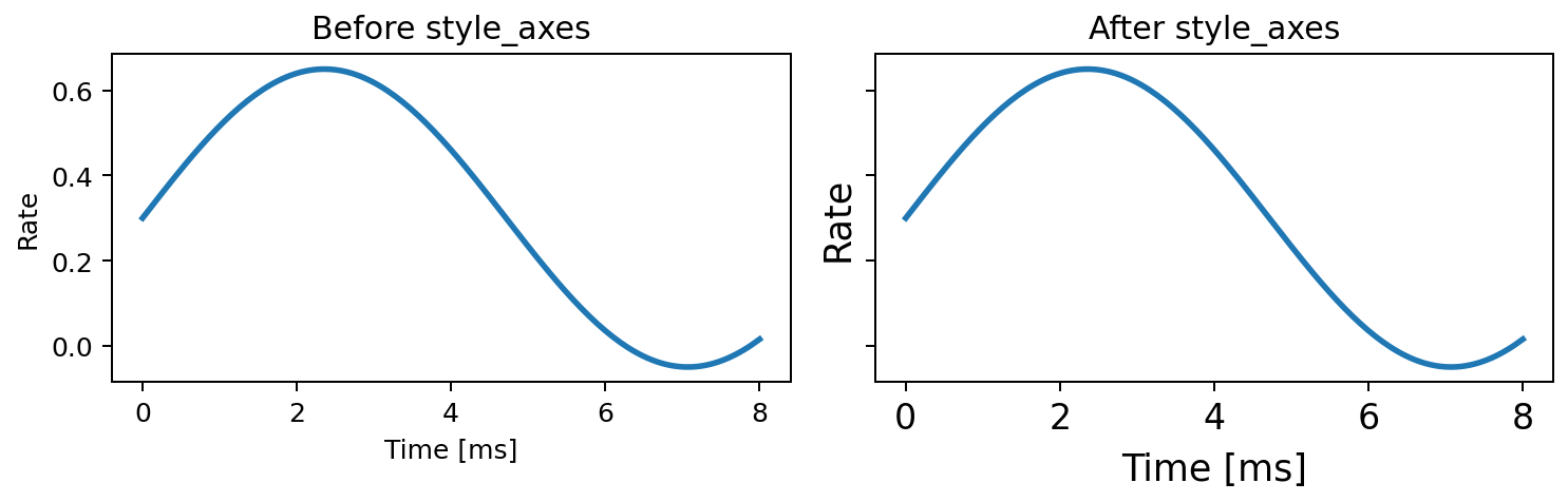 165 """ 166 if set_xlabel and ax.xaxis.label is not None: 167 ax.xaxis.label.set_size(fc.label) 168 ax.xaxis.labelpad = fc.labelpad 169 if set_ylabel and ax.yaxis.label is not None: 170 ax.yaxis.label.set_size(fc.label) 171 ax.tick_params(axis='both', labelsize=fc.tick)
Apply consistent label and tick font sizes to one axes.
Examples
fig, ax = plt.subplots()
ax.set_xlabel("Time [ms]")
ax.set_ylabel("Rate")
style_axes(ax, FontCfg().resolve())
Expected output
The x-label, y-label, and tick labels use the sizes defined by fc.

173def style_colorbar(cbar, fc: FontCfg, *, set_label=True): 174 """Apply consistent font sizes to a Matplotlib colorbar. 175 176 Expected output 177 --------------- 178 The colorbar label and tick labels use the sizes defined by `fc`. 179 180 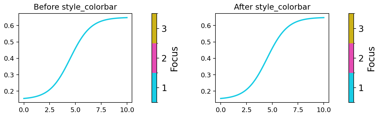 181 """ 182 if cbar is None: 183 return 184 ax = getattr(cbar, "ax", None) 185 if ax is None: 186 return 187 188 orient = getattr(cbar, "orientation", None) 189 if set_label: 190 if orient == "horizontal": 191 if ax.xaxis.label is not None: 192 ax.xaxis.label.set_size(fc.label) 193 ax.xaxis.labelpad = fc.labelpad 194 else: 195 if ax.yaxis.label is not None: 196 ax.yaxis.label.set_size(fc.label) 197 198 ax.tick_params(axis="both", labelsize=fc.tick)
Apply consistent font sizes to a Matplotlib colorbar.
Expected output
The colorbar label and tick labels use the sizes defined by fc.

201def style_legend(ax, fc: FontCfg): 202 """Apply the configured legend font size to an axes legend, if present. 203 204 Expected output 205 --------------- 206 All legend labels on the axes use `fc.legend`. 207 208 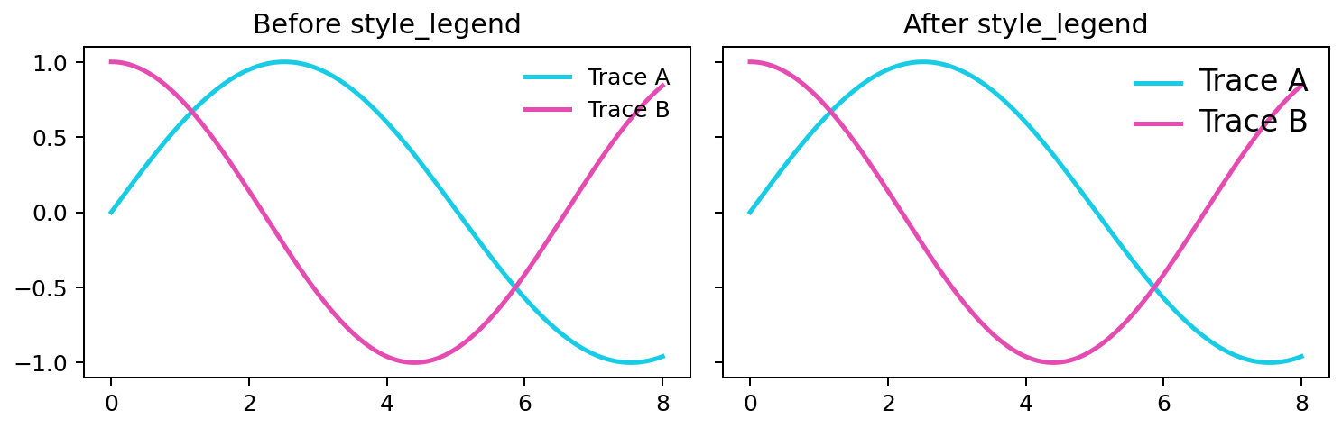 209 """ 210 leg = ax.get_legend() 211 if leg is not None: 212 for t in leg.get_texts(): 213 t.set_fontsize(fc.legend)
Apply the configured legend font size to an axes legend, if present.
Expected output
All legend labels on the axes use fc.legend.

135def compute_discrete_boundaries(values: Sequence[float]) -> List[float]:
136    """Compute colorbar boundaries for a discrete set of values.
137
138    Examples
139    --------
140    >>> compute_discrete_boundaries([1.0, 2.0, 4.0])
141    [0.5, 1.5, 3.0, 5.0]
142    """
143    numeric = [float(value) for value in values if value is not None]
144    if not numeric:
145        return []
146    ordered = sorted(dict.fromkeys(numeric))
147    if len(ordered) == 1:
148        val = float(ordered[0])
149        return [val - 0.5, val + 0.5]
150    gaps = [next_val - prev_val for prev_val, next_val in zip(ordered[:-1], ordered[1:])]
151    first_gap = gaps[0]
152    last_gap = gaps[-1]
153    boundaries = [ordered[0] - first_gap / 2.0]
154    for prev_val, next_val in zip(ordered[:-1], ordered[1:]):
155        midpoint = (prev_val + next_val) / 2.0
156        boundaries.append(midpoint)
157    boundaries.append(ordered[-1] + last_gap / 2.0)
158    return boundaries
Compute colorbar boundaries for a discrete set of values.
Examples
>>> compute_discrete_boundaries([1.0, 2.0, 4.0])
[0.5, 1.5, 3.0, 5.0]
161def draw_listed_colorbar( 162 fig: "Figure", 163 axis: "Axes", 164 entries: Sequence[Tuple[float, str]], 165 *, 166 font_cfg: "FontCfg", 167 label: str, 168 orientation: str = "vertical", 169 height_fraction: Optional[float] = None, 170 width_fraction: Optional[float] = None, 171 use_parent_axis: bool = False, 172 label_kwargs: Optional[Mapping[str, Any]] = None, 173): 174 """Draw a discrete listed colorbar from `(value, color)` entries. 175 176 Examples 177 -------- 178 ```python 179 fig, (ax, cax) = plt.subplots( 180 1, 181 2, 182 figsize=(4, 1.5), 183 gridspec_kw={"width_ratios": [4, 1]}, 184 ) 185 ax.plot([0, 1], [0, 1], color=LINE_COLORS[0]) 186 draw_listed_colorbar( 187 fig, 188 cax, 189 entries=[(1.0, LINE_COLORS[0]), (2.0, LINE_COLORS[1])], 190 font_cfg=FontCfg().resolve(), 191 label="Focused clusters", 192 ) 193 ``` 194 195 Expected output 196 --------------- 197 The second axes contains a two-level discrete colorbar with ticks at `1.0` 198 and `2.0`. 199 200 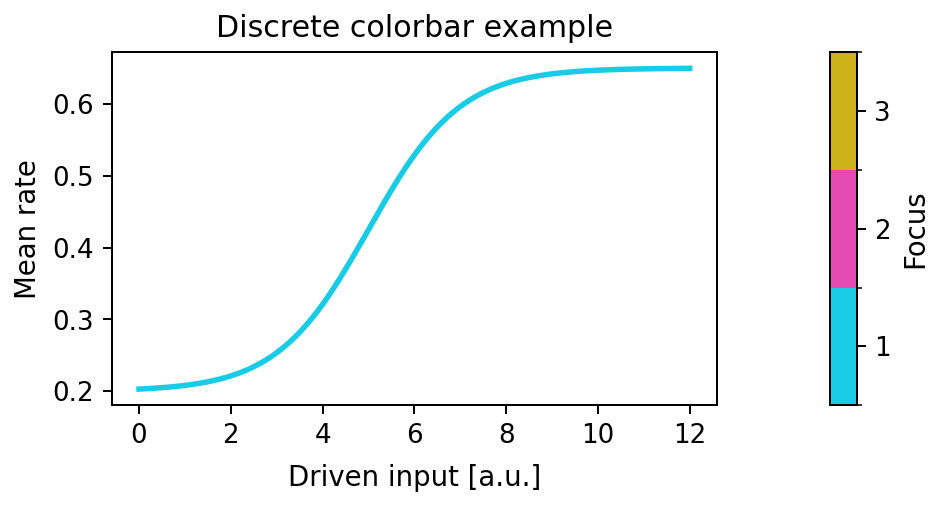 201 """ 202 if not entries: 203 axis.set_axis_off() 204 return None 205 ticks = [float(value) for value, _ in entries] 206 colors = [color for _, color in entries] 207 cmap = mcolors.ListedColormap(colors) 208 boundaries = compute_discrete_boundaries(ticks) 209 if len(boundaries) < 2: 210 single = ticks[0] if ticks else 0.0 211 boundaries = [single - 0.5, single + 0.5] 212 norm = mcolors.BoundaryNorm(boundaries, cmap.N) 213 scalar = plt.cm.ScalarMappable(norm=norm, cmap=cmap) 214 scalar.set_array([]) 215 colorbar_kwargs: Dict[str, Any] = { 216 "ticks": ticks, 217 "boundaries": boundaries, 218 "orientation": orientation, 219 } 220 if use_parent_axis: 221 colorbar_kwargs["ax"] = axis 222 else: 223 target_axis: "Axes" = axis 224 inset = [0.0, 0.0, 1.0, 1.0] 225 use_inset = False 226 effective_width_fraction = width_fraction 227 if effective_width_fraction is None and orientation == "vertical": 228 effective_width_fraction = 0.25 229 if height_fraction is not None and 0.0 < height_fraction < 1.0: 230 inset_height = height_fraction 231 inset[1] = (1.0 - inset_height) / 2.0 232 inset[3] = inset_height 233 use_inset = True 234 if effective_width_fraction is not None and 0.0 < effective_width_fraction < 1.0: 235 inset[0] = (1.0 - effective_width_fraction) / 2.0 236 inset[2] = effective_width_fraction 237 use_inset = True 238 if use_inset: 239 axis.set_axis_off() 240 target_axis = axis.inset_axes(inset) 241 colorbar_kwargs["cax"] = target_axis 242 colorbar = fig.colorbar(scalar, **colorbar_kwargs) 243 colorbar.ax.tick_params(labelsize=font_cfg.tick) 244 if label: 245 params = dict(label_kwargs or {}) 246 if orientation == "vertical": 247 colorbar.ax.set_ylabel(label, fontsize=font_cfg.label, **params) 248 else: 249 colorbar.ax.set_xlabel(label, fontsize=font_cfg.label, **params) 250 return colorbar
Draw a discrete listed colorbar from (value, color) entries.
Examples
fig, (ax, cax) = plt.subplots(
    1,
    2,
    figsize=(4, 1.5),
    gridspec_kw={"width_ratios": [4, 1]},
)
ax.plot([0, 1], [0, 1], color=LINE_COLORS[0])
draw_listed_colorbar(
    fig,
    cax,
    entries=[(1.0, LINE_COLORS[0]), (2.0, LINE_COLORS[1])],
    font_cfg=FontCfg().resolve(),
    label="Focused clusters",
)
Expected output
The second axes contains a two-level discrete colorbar with ticks at 1.0
and 2.0.
